| Issue |
A&A
Volume 516, June-July 2010
|
|
|---|---|---|
| Article Number | A64 | |
| Number of page(s) | 13 | |
| Section | Planets and planetary systems | |
| DOI | https://doi.org/10.1051/0004-6361/201014337 | |
| Published online | 29 June 2010 | |
Is tidal heating sufficient to explain bloated exoplanets? Consistent calculations accounting for finite initial eccentricity
J. Leconte1 - G. Chabrier1 - I. Baraffe1,2 - B. Levrard1
1 - École Normale Supérieure de Lyon, 46 allée d'Italie, 69364 Lyon
Cedex 07; Université Lyon 1, Villeurbanne, 69622; CNRS, UMR 5574,
Centre de Recherche Astrophysique de Lyon, France
2 - School of Physics, University of Exeter, Stocker Road, Exeter EX4
4PE, UK
Received 1 March 2010 / Accepted 3 April 2010
Abstract
We present the consistent evolution of short-period exoplanets coupling
the tidal and gravothermal evolution of the planet. Contrarily to
previous similar studies, our calculations are based on the complete
tidal evolution equations of the Hut (1981) model, valid at any order
in eccentricity, obliquity and spin. We demonstrate both
analytically and numerically that except if the system was formed
with a nearly circular orbit (![]() ), consistently solving the
complete tidal equations is mandatory to derive correct tidal evolution
histories. We show that calculations based on tidal models truncated at
2nd order in eccentricity, as done in all previous studies,
lead to quantitatively and sometimes even qualitatively erroneous tidal
evolutions. As a consequence, tidal energy dissipation rates are
severely underestimated in all these calculations and the
characteristic
timescales for the various orbital parameters evolutions can be wrong
by up to three orders of magnitude. These discrepancies can by no means
be justified by
invoking the uncertainty in the tidal quality factors.
), consistently solving the
complete tidal equations is mandatory to derive correct tidal evolution
histories. We show that calculations based on tidal models truncated at
2nd order in eccentricity, as done in all previous studies,
lead to quantitatively and sometimes even qualitatively erroneous tidal
evolutions. As a consequence, tidal energy dissipation rates are
severely underestimated in all these calculations and the
characteristic
timescales for the various orbital parameters evolutions can be wrong
by up to three orders of magnitude. These discrepancies can by no means
be justified by
invoking the uncertainty in the tidal quality factors.
Based on these complete, consistent calculations, we revisit the viability of the tidal heating hypothesis to explain the anomalously large radius of transiting giant planets. We show that even though tidal dissipation does provide a substantial contribution to the planet's heat budget and can explain some of the moderately bloated hot-Jupiters, this mechanism can not explain alone the properties of the most inflated objects, including HD 209 458 b. Indeed, solving the complete tidal equations shows that enhanced tidal dissipation and thus orbit circularization occur too early during the planet's evolution to provide enough extra energy at the present epoch. In that case either a third, so far undetected, low-mass companion must be present to keep exciting the eccentricity of the giant planet, or other mechanisms - stellar irradiation induced surface winds dissipating in the planet's tidal bulges and thus reaching the convective layers, inefficient flux transport by convection in the planet's interior - must be invoked, together with tidal dissipation, to provide all the pieces of the abnormally large exoplanet puzzle.
Key words: brown dwarfs - planet-star interactions - planets and satellites: dynamical evolution and stability - planets and satellites: general
1 Introduction
Gravitational tides have marked out the history of science and astrophysics since the first assessment by Seleucus of Seleucia of the relation between the height of the tides and the position of the moon and the Sun in the second century BC. Modern astrophysics extended the study of gravitational tides in an impressive variety of contexts from the synchronization of the Moon and other satellites to the evolution of close binary stars and even the disruption of galaxies.
The recent discoveries of short period extrasolar planetary
systems and the determination of the anomalously large radius of some
giant close-in exoplanets revived the need for a theory of planetary
tides covering a wider variety of orbital configurations than
previously encountered in our own solar system planets. In particular,
the orbital evolution of planetary systems like
HD 80 606, with an orbital eccentricity of 0.9337 (Naef et al. 2001), and
XO-3, with a stellar obliquity ![]() deg
(Winn et al. 2009b),
cannot be properly treated with tidal models limited to the case of
zero or vanishing eccentricity and obliquity as in the models of e.g. Goldreich & Soter (1966), Jackson et al. (2008) and Ferraz-Mello et al. (2008).
deg
(Winn et al. 2009b),
cannot be properly treated with tidal models limited to the case of
zero or vanishing eccentricity and obliquity as in the models of e.g. Goldreich & Soter (1966), Jackson et al. (2008) and Ferraz-Mello et al. (2008).
Following Bodenheimer et al. (2001) and Gu et al. (2003), attempts have been made to explain the observed large radius of some transiting close-in gas giant exoplanets - the so-called ``Hot Jupiters'' - by means of tidal heating (Ibgui et al. 2009; Jackson et al. 2008; Miller et al. 2009). All these models, however, use tidal models truncated to a low (2nd) order in eccentricity, in spite of initial eccentricities, as determined from the tidal evolution calculations, which can be as large as e=0.8! According to these calculations, a large eccentricity can remain long enough to lead to tidal energy dissipation in the planet's gaseous envelope (assuming a proper dissipation mechanism is at play in the deep convective layers) at a late epoch and then can explain the actual bloated radius of some observed planets.
In the present paper we revisit the viability of this tidal heating hypothesis, using an extended version of the Hut (1981) tidal evolution model, consistently solving the complete tidal equations, to any order in eccentricity and obliquity, and coupling these later with the gravothermal evolution of the irradiated planet. As will be shown, properly taking into account the full nature of the tidal equations severely modifies the planet's tidal and thermal evolution, compared with the aforementioned truncated calculations, which in turn leads to significantly different tidal heat rates and thus planet contraction rates.
After introducing our model in Sect. 2, we examine in
detail in Sect. 3
the relation between the constant time lag (![]() )
in Hut's (and thus our) model and the usual tidal quality
factor (Q) widely used in the literature.
Constraints on
)
in Hut's (and thus our) model and the usual tidal quality
factor (Q) widely used in the literature.
Constraints on ![]() from the study of the Galilean satellites are also derived. In
Sect. 4
we demonstrate with analytical arguments that
truncating the tidal equations at 2nd order in eccentricity
leads to wrong tidal evolution histories, with sequences drastically
differing from those obtained when solving the complete equations. In
Sect. 5,
we compare our full thermal/orbital evolution calculations with similar
studies based on a truncated and constant Q tidal
model. These numerical comparisons confirm and quantify the conclusions
reached
in Sect. 4,
namely that low-order eccentricity models substantially underestimate
the tidal evolution timescales for initially eccentric systems and thus
lead to
incorrect tidal energy contributions to the planet's energy balance. We
show for instance that tidal heating cannot explain the radius of
HD 209 458 b for the present values of their
orbital parameters, contrarily to what has been claimed in previous
calculations based on truncated eccentricity models (Ibgui
et al. 2009). Finally we apply our model in
Sect. 6
to some of the discovered bloated planets. We show that although tidal
heating can explain the presently observed radius of some moderately
bloated Hot Jupiters, as indeed suggested in some previous
studies, tidal heating alone cannot explain all the
anomalously large radii. Indeed, in these cases eccentricity damping
occurs too early in the system's tidal evolution (assuming a genuine
two-body planetary system) to lead to the present state of the planet's
contraction.
from the study of the Galilean satellites are also derived. In
Sect. 4
we demonstrate with analytical arguments that
truncating the tidal equations at 2nd order in eccentricity
leads to wrong tidal evolution histories, with sequences drastically
differing from those obtained when solving the complete equations. In
Sect. 5,
we compare our full thermal/orbital evolution calculations with similar
studies based on a truncated and constant Q tidal
model. These numerical comparisons confirm and quantify the conclusions
reached
in Sect. 4,
namely that low-order eccentricity models substantially underestimate
the tidal evolution timescales for initially eccentric systems and thus
lead to
incorrect tidal energy contributions to the planet's energy balance. We
show for instance that tidal heating cannot explain the radius of
HD 209 458 b for the present values of their
orbital parameters, contrarily to what has been claimed in previous
calculations based on truncated eccentricity models (Ibgui
et al. 2009). Finally we apply our model in
Sect. 6
to some of the discovered bloated planets. We show that although tidal
heating can explain the presently observed radius of some moderately
bloated Hot Jupiters, as indeed suggested in some previous
studies, tidal heating alone cannot explain all the
anomalously large radii. Indeed, in these cases eccentricity damping
occurs too early in the system's tidal evolution (assuming a genuine
two-body planetary system) to lead to the present state of the planet's
contraction.
2 Model description
2.1 Internal evolution
The main physics inputs (equations of state, internal composition, irradiated atmosphere models, boundary conditions) used in the present calculations have been described in detail in previous papers devoted to the evolution of extrasolar giant planets (Leconte et al. 2009; Baraffe et al. 2008,2003) and are only briefly outlined below. The evolution of the planet is based on a consistent treatment between the outer non-grey irradiated atmospheric structure and the inner structure. The interior is composed primarily of a gaseous H/He envelope whose thermodynamic properties are described by the Saumon-Chabrier-VanHorn equation of state (EOS, Saumon et al. 1995) with a solar or non-solar enrichment in heavy elements described by the appropriate EOS's (Baraffe et al. 2008). In the present calculations, our fiducial model consists of a planet with a central core made up of water, with the ANEOS EOS (Thompson & Lauson 1972). A detailed analysis of the effects of different EOS's, core compositions and heavy material repartitions within the planet can be found in Baraffe et al. (2008), as well as a comparison with models from other groups, in particular those by Fortney et al. (2007).
Transiting planets are by definition very close to their host
star (a< 0.1 AU).
In that case, the stellar irradiation strongly affects the planet
atmospheric structure to deep levels (Barman
et al. 2001)
and thus the planet's evolution (Guillot
et al. 1996; Baraffe
et al. 2003; Burrows
et al. 2003; Chabrier
et al. 2004; Leconte
et al. 2009). We use a grid of irradiated atmosphere
models based on the calculations of
Barman et al. (2001),
computed for different levels of stellar irradiation relevant
to the present study. For planets with a finite orbital eccentricity,
the mean stellar flux received is given by

where
2.2 Tidal model
We consider the gravitational tides raised by both the host star and
the planet on each other and follow the traditional ``viscous''
approach of the
equilibrium tide theory (Darwin
1908). The secular evolution of the semi-major axis a
can be calculated exactly (e.g. Hut 1981;
Neron de Surgy & Laskar 1997;
Levrard et al. 2007; Correia & Laskar 2010; see
Appendix A
for the derivation of these equations for any value of the eccentricity
and obliquity)
with
and

where G is the gravitational constant,

|
(5) |
where
![$\displaystyle 11\frac{a}{GM_{\star}M_{\rm p}}
\left\{K_{{\rm p}}\left[\Omega_{e}(e)~x_{\rm p}~
\frac{\omega_{\rm p}}{n}-\frac{18}{11}N_{e}(e)\right] \right.$](/articles/aa/full_html/2010/08/aa14337-10/img41.png)
![$\displaystyle \left.\qquad ~~~ \qquad +K_{\star}\left[\Omega_{e}(e)~x_\star~
\frac{\omega_\star}{n}-\frac{18}{11}N_{e}(e)\right]\right\},$](/articles/aa/full_html/2010/08/aa14337-10/img42.png)
with

and

The terms proportional to
![\begin{displaymath}\frac{{\rm d}C_{\rm i}\omega_{\rm i}}{{\rm d}t}=-\frac{K_{\rm...
...t)\Omega(e)\frac{\omega_{\rm i}}{n}-2x_{\rm i}~N(e)
\right] ,
\end{displaymath}](/articles/aa/full_html/2010/08/aa14337-10/img47.png)
while the evolution of the obliquity obeys the equation
![\begin{displaymath}\frac{{\rm d}\varepsilon_{\rm i}}{{\rm d}t}=\sin \varepsilon_...
..._{\rm i})~\Omega(e) \frac{\omega_{\rm i}}{n}- 2~N(e) \right] ,
\end{displaymath}](/articles/aa/full_html/2010/08/aa14337-10/img48.png)
where

and

Up to this point, no assumption has been made on the objects themselves. As a result, Eqs. (2)-(10) are fully symmetric in p and
within a time scale
![\begin{displaymath}\dot{E}_{{\rm tides}}=
2K_{{\rm p}}\left[N_{a}(e)-\frac{N^2(e)}{\Omega(e)} \right] ;\ \ (\omega_{\rm p}=\omega_{{\rm eq}}) .
\end{displaymath}](/articles/aa/full_html/2010/08/aa14337-10/img58.png)
The dissipated heat is deposited over the whole planet's interior.
One can see from Eq. (A.26) in
Appendix A
that Eq. (13)
is a special case of energy dissipation for a body in
pseudo-synchronous rotation as expected for fluid objects (
![]() ,
,
![]() ).
For a rocky planet, the external gravitational potential created by its
permanent quadrupole moment can cause its locking into synchronous
rotation (
).
For a rocky planet, the external gravitational potential created by its
permanent quadrupole moment can cause its locking into synchronous
rotation (
![]() ), and the dissipation rate
reads in that case
), and the dissipation rate
reads in that case
![$\displaystyle \dot{E}_{{\rm tides}}=2~K_{{\rm p}}
\left[N_{a}(e)-2 N(e)~x_{\rm p}+\left(\frac{1+x_{\rm p}^2}{2}\right)\Omega(e)\right] ;\ (\omega_{\rm p}=n) .$](/articles/aa/full_html/2010/08/aa14337-10/img60.png)
|
(14) |
This equation fully agrees with Eq. (30) of Wisdom (2008) who calculated it for a homogeneous, incompressible with a radial displacement Love number h2 =5k2/3. Note that our derivation does not require such an hypothesis and all the uncertainties in the radial distribution of material and its physical properties (e.g., density, compressibility, elasticity) are lumped into the k2 parameter (Levrard 2008).
3 Relationship between the time lag  t and the
quality factor (Q)
t and the
quality factor (Q)
The aforedescribed tidal model, which leads to exact
tidal evolution equations in the viscous approximation, implies a constant
time lag ![]() .
Neither the tidal quality factor (Q) or its
counterpart, the phase lag (
.
Neither the tidal quality factor (Q) or its
counterpart, the phase lag (![]() )
(Goldreich
& Soter 1966; Goldreich 1963) enter the dynamical
evolution equations. Instead, the model is characterized by the time
lag between the maximum of the tidal potential and the tidal bulge in
each body,
)
(Goldreich
& Soter 1966; Goldreich 1963) enter the dynamical
evolution equations. Instead, the model is characterized by the time
lag between the maximum of the tidal potential and the tidal bulge in
each body, ![]() ,
considered to be constant during the evolution. As shown e.g. by Darwin (1908, see also Greenberg 2009), this
model is equivalent to considering a body whose rheology entails
,
considered to be constant during the evolution. As shown e.g. by Darwin (1908, see also Greenberg 2009), this
model is equivalent to considering a body whose rheology entails ![]() ,
where
,
where ![]() is the frequency of the tidal forcing. The actual rheology of giant
gaseous planets being poorly constrained, this arbitrary choice based
on the visco-elastic model has the advantages of (i) not
introducing any discontinuity for vanishing tidal frequencies, as is
the case for synchronous rotation, and (ii) to allow for a complete
calculation of the tidal effect without any assumption on the
eccentricity for an ideal viscoelastic body.
is the frequency of the tidal forcing. The actual rheology of giant
gaseous planets being poorly constrained, this arbitrary choice based
on the visco-elastic model has the advantages of (i) not
introducing any discontinuity for vanishing tidal frequencies, as is
the case for synchronous rotation, and (ii) to allow for a complete
calculation of the tidal effect without any assumption on the
eccentricity for an ideal viscoelastic body.
Indeed, as shown by Greenberg
(2009), the frequency dependence of the phase lag of a
perfect viscoelastic oscillator is given by

|
(15) |
where

|
(16) |
which is the frequency dependence corresponding to the constant time-lag model.
On the contrary, constant-Q models
described by Goldreich & Soter
(1966), Jackson
et al. (2008), Ferraz-Mello
et al. (2008) were derived using perturbative
developments of Kepler equations of motion both in eccentricity and
inclination. Such Fourier decomposition is indeed necessary in a ``lag
and add'' approach with a given frequency-dependence of the phase lag (
![]() ). Indeed, in this approach,
one must first separate the forcing potential in terms with a defined
frequency before lagging them with the chosen
). Indeed, in this approach,
one must first separate the forcing potential in terms with a defined
frequency before lagging them with the chosen ![]() (see Ferraz-Mello
et al. 2008; Greenberg 2009). As a result they
can only be used in the
(see Ferraz-Mello
et al. 2008; Greenberg 2009). As a result they
can only be used in the ![]() and
and ![]() limit.
limit.
The time lag ![]() can be linked to the reduced quality factor
can be linked to the reduced quality factor ![]() ,
chosen so that Q'=Q for a
homogeneous sphere (k2=3/2).
Indeed, one must remember that the phase lag,
,
chosen so that Q'=Q for a
homogeneous sphere (k2=3/2).
Indeed, one must remember that the phase lag, ![]() ,
induced by the
tidal dissipative effects, is twice the geometrical lag angle,
,
induced by the
tidal dissipative effects, is twice the geometrical lag angle, ![]() ,
between the maximum of the deforming potential and the tidal bulge:
,
between the maximum of the deforming potential and the tidal bulge: ![]() .
Moreover, for an incompressible body, a reasonable assumption for giant
planets, the tidal dissipation function is given by (Goldreich 1963;
Efroimsky
& Williams 2009)
.
Moreover, for an incompressible body, a reasonable assumption for giant
planets, the tidal dissipation function is given by (Goldreich 1963;
Efroimsky
& Williams 2009)

where

This formula can be used to estimate the quality factor for jovian planets as long as semi-diurnal tides dominate. As the planet tends toward synchronization, the dissipative effects of the semi diurnal tides (

Apart from these two limit cases, no tidal frequency dominates, and the dissipation is the response of the body to the rich spectrum of exciting tidal frequencies. Thus no simple relation exists between Q' and
Although it is tempting to use Eq. (19) to rewrite the
tidal equation and to keep Q' constant instead of ![]() as done by, for example, Mardling
& Lin (2002), Dobbs-Dixon
et al. (2004) and Barker
& Ogilvie (2009), one must keep in mind that this
procedure is not equivalent either to the constant phase lag (i.e.
constant Q) or time lag model. Indeed the frequency
dependence of the phase lag is given by
as done by, for example, Mardling
& Lin (2002), Dobbs-Dixon
et al. (2004) and Barker
& Ogilvie (2009), one must keep in mind that this
procedure is not equivalent either to the constant phase lag (i.e.
constant Q) or time lag model. Indeed the frequency
dependence of the phase lag is given by ![]() and is still proportional to the tidal frequency over an orbit as in
the constant time-lag model, but with a slope that is changing during
the evolution.
and is still proportional to the tidal frequency over an orbit as in
the constant time-lag model, but with a slope that is changing during
the evolution.
In Sects. 4
and 5,
we compare the constant time-lag model with the constant Q'
model used by various authors. In order to allow a direct and immediate
comparison with these studies, we will choose the values of the couple ![]() from the relations
from the relations ![]() ,
where
,
where ![]() are the constant normalized quality factors used by
Miller et al. (2009).
This ensures that the effective tidal dissipation function is the same
in both calculations for a given planet with its measured orbital
parameters.
are the constant normalized quality factors used by
Miller et al. (2009).
This ensures that the effective tidal dissipation function is the same
in both calculations for a given planet with its measured orbital
parameters.
In order to use the constant time lag
model, we must consider many values for ![]() .
To constrain this parameter, we follow the analysis of Goldreich & Soter (1966) and
use the Io-Jupiter system to infer an upper limit for
.
To constrain this parameter, we follow the analysis of Goldreich & Soter (1966) and
use the Io-Jupiter system to infer an upper limit for ![]() in giant extrasolar planets. Because Jupiter is rapidly rotating, with
in giant extrasolar planets. Because Jupiter is rapidly rotating, with ![]() (hereafter, J indices refer to the value for Jupiter), where n
is the orbital mean motion of Jupiter's satellites, tidal transfer of
angular momentum drives the satellites of Jupiter
outwards, into expanding orbits. Therefore the
presence of Io in a close orbit provides an upper limit for the time
lag in Jupiter. Indeed, if
(hereafter, J indices refer to the value for Jupiter), where n
is the orbital mean motion of Jupiter's satellites, tidal transfer of
angular momentum drives the satellites of Jupiter
outwards, into expanding orbits. Therefore the
presence of Io in a close orbit provides an upper limit for the time
lag in Jupiter. Indeed, if ![]() was too large, the backward evolution of the satellites' orbits would
imply their disappearance within less time than the age of the Solar
system, i.e. of Jupiter.
For coplanar and circular orbits a dimensionless version of
Eq. (2)
reads
was too large, the backward evolution of the satellites' orbits would
imply their disappearance within less time than the age of the Solar
system, i.e. of Jupiter.
For coplanar and circular orbits a dimensionless version of
Eq. (2)
reads
![\begin{displaymath}
\dot{\tilde{a}}=- \frac{1}{\tilde{a}^7}\left[1 -\frac{\omega_\star}{n}\right],
\end{displaymath}](/articles/aa/full_html/2010/08/aa14337-10/img91.png)
where

where

into Eq. (20), and integrating over time yields
![\begin{displaymath}
\int_1^{\frac{a(t)}{a_0}} \frac{-\tilde{a}^7 {\rm d}\tilde{a...
...}-\beta\left(\sqrt{\tilde{a}}-1\right)\right]}=\frac{t}{\tau},
\end{displaymath}](/articles/aa/full_html/2010/08/aa14337-10/img96.png)
where
For the Io-Jupiter system, taking ![]() yr
and a(t) equal to the Roche
limit in Eq. (21)
yields
yr
and a(t) equal to the Roche
limit in Eq. (21)
yields ![]() s.
Therefore Eq. (18)
implies
s.
Therefore Eq. (18)
implies ![]() for the actual Io-Jupiter system, slightly lower than the value derived
by Goldreich & Soter (1966).
As discussed by these authors, our upper limit on
for the actual Io-Jupiter system, slightly lower than the value derived
by Goldreich & Soter (1966).
As discussed by these authors, our upper limit on
![]() must be multiplied by a factor 5 to 7.5, as Io might have been
trapped in a low order commensurability with Europa and Ganymede during
part of its evolution, slowing down the expansion of its orbit. This
roughly yields
must be multiplied by a factor 5 to 7.5, as Io might have been
trapped in a low order commensurability with Europa and Ganymede during
part of its evolution, slowing down the expansion of its orbit. This
roughly yields
For the sake of easy comparison, we will refer to the quantity Q'0, which is the reduced quality factor computed for a reference period of one day:

The above calculated constraint reads
It is important to stress that if ![]() ,
or its counterpart Q, is poorly known for both
planets and stars, its variability from one object or configuration to
another is even more uncertain. For instance, the tidal dissipation in
planets probably differs significantly from that in brown dwarfs
because of a dense core able to excite inertial waves in the convective
envelope (Goodman & Lackner 2009).
Given the highly
non-linear behavior of tidal dissipation mechanisms, the effective
tidal dissipation function varies not only with the structure of the
object or with
the tidal frequency, but also with the amplitude of the tidal
potential. For example,
,
or its counterpart Q, is poorly known for both
planets and stars, its variability from one object or configuration to
another is even more uncertain. For instance, the tidal dissipation in
planets probably differs significantly from that in brown dwarfs
because of a dense core able to excite inertial waves in the convective
envelope (Goodman & Lackner 2009).
Given the highly
non-linear behavior of tidal dissipation mechanisms, the effective
tidal dissipation function varies not only with the structure of the
object or with
the tidal frequency, but also with the amplitude of the tidal
potential. For example, ![]() values
inferred from the circularization of close FGK binary stars (Meibom & Mathieu 2005), may
be lower than the actual
values
inferred from the circularization of close FGK binary stars (Meibom & Mathieu 2005), may
be lower than the actual ![]() encountered in star-planet systems (Ogilvie
& Lin 2007). Consequently, the range of values
considered here for both
encountered in star-planet systems (Ogilvie
& Lin 2007). Consequently, the range of values
considered here for both ![]() and
and ![]() should be seen as mean values and be re-evaluated when considering
specific and/or atypical systems (XO-3, HAT-P-2 or CoRoT-Exo-3 for
example).
should be seen as mean values and be re-evaluated when considering
specific and/or atypical systems (XO-3, HAT-P-2 or CoRoT-Exo-3 for
example).
4 Effect of the truncation of the tidal equations to 2nd order in e: analytical analysis
Following the initial studies of Jackson
et al. (2008), all studies exploring the effect of
tidal heating on the internal evolution of ``Hot Jupiters'' (Miller et al. 2009; Ibgui et al. 2009) have
been using a tidal model assuming a constant Q value
during the evolution. Moreover, in all these calculations the tidal
evolution
equations are truncated at the 2nd order in eccentricity
(hereafter referred to as the ``e2
model''), even when considering tidal evolution
sequences with non-negligible values of e at
earlier stages of evolution. Although such a e2-truncated
model is justified for planets and satellites in the solar system (Goldreich &
Soter 1966; Kaula
1963), it becomes invalid, and thus yields incorrect results
for a(t), e(t)
and ![]() for finite eccentricity values. The main argument claimed for using
this simple tidal model is the large uncertainty on the tidal
dissipation processes in astrophysical objects. In particular, as
detailed by Greenberg (2009),
the linearity of the response to the tidal forcing based on the
viscoelastic model may not hold in a real object for the large spectrum
of exciting frequencies encountered when computing high-order terms in
the eccentricity. Although the large uncertainty in the dissipative
processes certainly precludes an exact determination of the tidal
evolution, it can by no means justify calculations which are neglecting
dominant terms at finite e.
for finite eccentricity values. The main argument claimed for using
this simple tidal model is the large uncertainty on the tidal
dissipation processes in astrophysical objects. In particular, as
detailed by Greenberg (2009),
the linearity of the response to the tidal forcing based on the
viscoelastic model may not hold in a real object for the large spectrum
of exciting frequencies encountered when computing high-order terms in
the eccentricity. Although the large uncertainty in the dissipative
processes certainly precludes an exact determination of the tidal
evolution, it can by no means justify calculations which are neglecting
dominant terms at finite e.
Indeed, from a dimensional point of view and prior to any
particular tidal model, the strong impact of high-order terms in the
eccentricity is simply caused by the tidal torque (![]() )
being proportional to
)
being proportional to ![]() (
(![]() being the true anomaly) and that over a Keplerian orbit the average
work done by the torque is of the form
being the true anomaly) and that over a Keplerian orbit the average
work done by the torque is of the form

which is a rapidly increasing function of e (see Appendix A for the details of the calculation). This means that although the mean distance between the planet and the star increases with e, the distance at the periapsis strongly decreases, and most of the work due to the tidal forces occurs at this point of the orbit. One can see that for e>0.32 the high-order terms dominate the constant and e2 terms. This is physical evidence that shows that for moderate to high eccentricity most of the tidal effects are contained in the high-order terms that can therefore not be neglected independently of any tidal model.
In this section we quantify this statement more comprehensively. We will demonstrate analytically that
- in the context of the Hut model, a truncation of the tidal equations at the order e2 can lead not only to quantitatively wrong but to qualititatively wrong tidal evolution histories, with sequences drastically differing from those obtained with the complete solution;
- the rate of tidal dissipation can be severely
underestimated by the quasi circular approximation (
 ).
).
4.1 Expanding vs. shrinking orbits
On one hand, considering Eq. (2) (with ![]() for simplification) we can see that for
for simplification) we can see that for ![]() ,
the tides raised on the body i lead to a
decrease of the semi-major axis, transferring the angular momentum from
the orbit to the body's internal rotation. It is easy to show that for
a synchronous planet this condition is always fulfilled, because
,
the tides raised on the body i lead to a
decrease of the semi-major axis, transferring the angular momentum from
the orbit to the body's internal rotation. It is easy to show that for
a synchronous planet this condition is always fulfilled, because ![]() for any eccentricity (respectively solid and dashed curves of
Fig. 1a).
As a result, the semi-major axis of most short period planets is
decreasing.
for any eccentricity (respectively solid and dashed curves of
Fig. 1a).
As a result, the semi-major axis of most short period planets is
decreasing.
![\begin{figure}% latex2html id marker 753\par\subfigure[$\omega/n$\space vs. $e...
...ted equations]{\includegraphics[width=7.5cm,clip]{14337fg1b.ps} }\end{figure}](/articles/aa/full_html/2010/08/aa14337-10/img127.png)
|
Figure 1:
Pseudo-synchronization curve (solid), the |
| Open with DEXTER | |
On the other hand, truncating Eq. (2) at the order e2
for the semi-major axis evolution yields
![$\displaystyle \frac{4~a}{GM_{\star}M_p}\left\{K_{{\rm p}}\left[\left(1+\frac{27}{2}e^2\right)
\frac{\omega_{\rm p}}{n}-\left(1+23~e^2\right)\right]\right.$](/articles/aa/full_html/2010/08/aa14337-10/img129.png)
![$\displaystyle \left. +K_{\star}\left[\left(1+\frac{27}{2}e^2\right)
\frac{\omega_\star}{n}-\left(1+23~e^2\right)\right]\right\},$](/articles/aa/full_html/2010/08/aa14337-10/img130.png)
and the previous condition becomes
This means that even for a moderate eccentricity,

and not to a decrease. This is illustrated by Fig. 1, which shows the pseudo-synchronization curve (solid), the
4.2 Underestimating tidal heating
The key quantity arising from the coupling between the orbital
evolution and the internal cooling history of a planet is the amount of
energy dissipated by the tides in the planet's interior, which may
compensate or even dominate its energy losses. As a result, tides
raised in an eccentric planet can slow down its contraction (Bodenheimer
et al. 2001; Baraffe et al. 2010; Leconte
et al. 2009) or even lead to a transitory phase of
expansion (Ibgui
et al. 2009; Miller et al. 2009).
Correctly determining
the tidal heating rate is thus a major issue in the evolution of
short-period planets. The often used formula is (Peale & Cassen 1978; Jackson
et al. 2008; Kaula 1963)
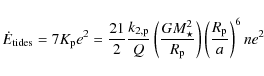
(the
![\begin{figure}
\par\includegraphics[width=7.8cm,clip]{14337fg2.ps}
\end{figure}](/articles/aa/full_html/2010/08/aa14337-10/img147.png)
|
Figure 2:
Tidal energy dissipation rate in a pseudo-synchronized planet (in Watt)
as a function of the eccentricity calculated with Eq. (13) (solid
curve) and with the truncated formula (Eq. (23); dashed).
The ratio of the two curves only depends on the eccentricity and not on
the system's parameters. For e=0.45, the e2
approximation (Eq. (23))
underestimates the tidal heating by a factor 10. The actual values were
derived using HD 209 458 b parameters: |
| Open with DEXTER | |
From a mathematical point of view, the fact that a truncation to
2nd order in eccentricity yields such discrepancies is due to
the ![]() factors in the equations for the tidal dissipation. As already stated
by Wisdom (2008), for moderate
to high eccentricity this function is poorly represented by the first
terms of its polynomial representation. Indeed, the first terms of the
energy dissipation rate are given by
factors in the equations for the tidal dissipation. As already stated
by Wisdom (2008), for moderate
to high eccentricity this function is poorly represented by the first
terms of its polynomial representation. Indeed, the first terms of the
energy dissipation rate are given by

The dissipation rate calculated up to e10 is plotted in Fig. 2 (dotted curve), where it can be compared with the exact result. It is clear that for
In particular, as discussed in the next section, a high
eccentricity (![]() )
cannot be maintained for a few 100 Myr to a few Gyr in a system like
HD 209 458 in agreement with the results of Miller et al. (2009) (see
Fig. 4
below).
This is in contrast with Ibgui &
Burrows (2009), who find that the radius
HD 209 458 b can be matched and that the
system can sustain a significant eccentricity up to the observed epoch.
These discrepancies between these two studies based on the same tidal
model may reveal differences in the implementations of the tidal
equations, or a difference in the calculation of interior structures or
boundary conditions.
)
cannot be maintained for a few 100 Myr to a few Gyr in a system like
HD 209 458 in agreement with the results of Miller et al. (2009) (see
Fig. 4
below).
This is in contrast with Ibgui &
Burrows (2009), who find that the radius
HD 209 458 b can be matched and that the
system can sustain a significant eccentricity up to the observed epoch.
These discrepancies between these two studies based on the same tidal
model may reveal differences in the implementations of the tidal
equations, or a difference in the calculation of interior structures or
boundary conditions.
5 Effect of the truncation to 2nd order in e: simulation results
In this section, we present the comparison of the results of our
complete model with the ``e2
model''. We calculated evolutionary tracks of the tidal evolution for
various transiting systems, coupling the internal evolution of the
object either with our tidal model or with the ``e2
model'' used in Miller et al.
(2009) and Ibgui &
Burrows (2009). In order to ensure a consistent comparison
with these authors, we directly convert their set of tidal parameters.
Because our model assumes a constant time lag, and not a constant Q' value,
a history track computed with the Q' ``e2 model''
with a constant couple (
![]() )
is compared with a history track computed in our model with a constant
couple
)
is compared with a history track computed in our model with a constant
couple ![]() given by
given by ![]() (see Sect. 3
and Eq. (19)).
This ensures that - although our calculations are conducted with a constant
(see Sect. 3
and Eq. (19)).
This ensures that - although our calculations are conducted with a constant
![]() - the quality factor computed with Eq. (19) in the object
at the present time is the same as that used in the Q
constant model.
- the quality factor computed with Eq. (19) in the object
at the present time is the same as that used in the Q
constant model.
5.1 Calculations at low eccentricity
![\begin{figure}
\par\subfigure[Semi-major axis]{\includegraphics[width=4cm,clip]{...
...phics[width=4cm,clip]{14337fg3d.ps} }
\vspace*{-2mm}\vspace*{2mm}
\end{figure}](/articles/aa/full_html/2010/08/aa14337-10/img155.png)
|
Figure 3:
Consistent tidal/thermal evolution of TrES-1 b computed with
our constant time-lag model (solid line) and with
the ``e2 model'' (dashed
line). This is a 0.76 |
| Open with DEXTER | |
We first compare the results of the two models on a system which has a zero measured eccentricity and is not inflated, namely TrES-1. Such a system does not require a substantial initial eccentricity for its observed properties to be reproduced and thus provides an opportunity to test the quasi-circular limit, where the ``e2 model'' used by Miller et al. (2009) and our model should yield similar results. Figure 3 illustrates the results of the integration of the coupled internal/orbital evolution equations with our constant time-lag model (solid curve) and with the ``e2 model'' (dashed curve) for an initial eccentricity of 0.07. As expected, in this low eccentricity limit both models yield very similar tracks: the eccentricity is damped to zero in a few Gyr and the semi-major axis decreases until the planet reaches the Roche limit and merges with the star, because the system does not have enough angular momentum to reach a stable equilibrium (Hut 1980; Levrard et al. 2009). In this case, tidal heating is not sufficient to significantly affect the radius of the planet, which keeps shrinking steadily as it cools. Note however that although the qualitative behavior of the evolution is the same, the hypothesis made on the rheology of the body can influence the age at which the merging occurs.
5.2 Calculations at high eccentricity
![\begin{figure}
\par\mbox{ \subfigure[Semi-major axis]{\includegraphics[width=4.1...
...rgy dissipation]{\includegraphics[width=4cm,clip]{14337fg4d.ps} }}\end{figure}](/articles/aa/full_html/2010/08/aa14337-10/img156.png)
|
Figure 4:
Consistent tidal/thermal evolution of XO-4 b (thin,
black) and HD 209 458 b (thick,
blue) computed with our constant time-lag model (solid
line) and with the ``e2 model''
(dashed line). XO-4 b is a 1.72 |
| Open with DEXTER | |
In the moderately to highly eccentric regime, the tidal dissipation rate can no longer be approximated by Eq. (23) (see Sect. 4.2). Instead, Eq. (13) must be used and yields - as shown by Fig. 2 - a much more important dissipation rate. As a result, tidal evolution takes place on a much shorter time scale, and both the eccentricity damping and the merging with the star occur earlier in the evolution of the planet. For illustration Fig. 4 portrays the possible thermal/tidal evolution (for given initial conditions) for XO-4 b (thin black curves) and HD 209 458 b (thick blue curves) computed with the ``e2 model'' (dashed) and with our model (solid). The dashed curves are similar to those displayed in Figs. 8 and 10 of Miller et al. (2009). As mentioned above and illustrated in Fig. 4d, the energy dissipation is much larger when fully accounting for the high eccentricity. The evolution of the planet can exhibit two different general behaviors:
- The planet first undergoes a phase of contraction and rapid
cooling before the tidal heating due to the high initial eccentricity
starts to dominate the energy balance of the object, leading to a phase
of radius inflation (as shown by Fig. 5 for a test
case).
This speeds up the damping of the eccentricity and the decrease of the semi-major axis, because
![\begin{figure}
\par\includegraphics[width=7.8cm,clip]{14337fg5.eps}\vspace*{-2mm}
\vspace*{2mm}
\end{figure}](/articles/aa/full_html/2010/08/aa14337-10/Timg157.png)
Figure 5: Internal energy balance in the evolving planet. Solid line: luminosity of the object with tidal heating. Dotted line: luminosity of the object without tidal heating. Dashed line: tidal energy dissipation rate. The object contracts as it cools until the energy input balances its thermal losses and sustains a higher entropy in the gaseous envelop, yielding a larger radius.
Open with DEXTER  and
and  .
When the eccentricity becomes ow enough, a ``standard'' contraction
phase begins and lasts until the planet merges with the star (due to stellar
tides; Levrard et al. 2009)
or - if enough angular momentum is present in the system - until both
tidal and thermal equilibria are achieved. This behavior has already
been identified by Miller
et al. (2009) and Ibgui
& Burrows (2009), but because these authors used
truncated tidal equations, they found that a high eccentricity can be
maintained for a few Gyr and kept inflating the planet at a late time,
as illustrated in Fig. 4
(dashed curves); while this is not the case.
.
When the eccentricity becomes ow enough, a ``standard'' contraction
phase begins and lasts until the planet merges with the star (due to stellar
tides; Levrard et al. 2009)
or - if enough angular momentum is present in the system - until both
tidal and thermal equilibria are achieved. This behavior has already
been identified by Miller
et al. (2009) and Ibgui
& Burrows (2009), but because these authors used
truncated tidal equations, they found that a high eccentricity can be
maintained for a few Gyr and kept inflating the planet at a late time,
as illustrated in Fig. 4
(dashed curves); while this is not the case.
- In some extreme cases like HD 209 458,
for the initial conditions corresponding to those in Fig. 4, the tidal
heating can overwhelm the cooling rate of the planet by orders of
magnitude and lead to a spectacular inflation of the planet and thus to
a rapid merging with the star. This stems from a combination of
different effects. First of all, as mentioned above, the expansion of
the radius accelerates the tidal evolution and thus the decrease of the
orbital distance. Furthermore, the Roche limit (
![$a_{\rm R}=\alpha R_{\rm p}\sqrt[3]{M_\star/ M_{\rm p}}$](/articles/aa/full_html/2010/08/aa14337-10/img160.png) ,
where
,
where  is a constant which depends on the structure of the body and is equal
to 2.422 for fluid objects) increases with the radius of the planet,
extending the merging zone.
is a constant which depends on the structure of the body and is equal
to 2.422 for fluid objects) increases with the radius of the planet,
extending the merging zone.
6 Global view of transiting systems
As mentioned earlier, tidal heating has been suggested by several authors to explain the anomalously large radius of some giant close-in observed exoplanets. As demonstrated in Sect. 5, the previous calculations, which are all based on constant-Q models truncated at the order e2 yield inaccurate results when applied to significantly (initial or actual) eccentric orbits - a common situation among detected exoplanetary systems. In this section, we revisit the viability of such a tidal heating mechanism to explain the extensive observed Hot Jupiter radii with the present complete Hut tidal model. We first examine the properties of the known transiting systems. Then we show that although it indeed provides a possible explanation for some transiting systems, the tidal heating hypothesis fails to explain the radii of extremely bloated planets like - among others - HD 209 458 b, TrES-4 b, WASP-4 b or WASP-12 b, in contrast with some previously published results based on truncated tidal models (see Sect. 7).
It is now well established that a large number of transiting
giant exoplanets are more inflated than predicted by the standard
cooling theory of irradiated gaseous giant planets (see Udry & Santos
2007; Baraffe
et al. 2010, for reviews).
In order to quantify this effect we computed the radius predicted by
our standard model, described in Sect. 2.1, for
the 54 transiting planets detected at the time of writing of
this paper, with ![]() (about a Saturn mass). We define the radius excess
as the difference between the observed radius and that predicted by the
model at the estimated age of the system, denominated
(about a Saturn mass). We define the radius excess
as the difference between the observed radius and that predicted by the
model at the estimated age of the system, denominated ![]() .
Results are summarized in Fig. 6. The
existence of objects below the
.
Results are summarized in Fig. 6. The
existence of objects below the ![]() line is a clear signature of a dense core and/or of the enrichment of
the gaseous envelope (Fortney
et al. 2007; Leconte et al. 2009; Baraffe
et al. 2008; Burrows et al. 2007; Baraffe
et al. 2006). Note that most of the objects
significantly below this line are in the
line is a clear signature of a dense core and/or of the enrichment of
the gaseous envelope (Fortney
et al. 2007; Leconte et al. 2009; Baraffe
et al. 2008; Burrows et al. 2007; Baraffe
et al. 2006). Note that most of the objects
significantly below this line are in the ![]() region and can be explained with a
region and can be explained with a ![]() heavy material enrichment (Baraffe
et al. 2008), in good agreement with predictions of
the core-accretion scenario for planet formation (Mordasini
et al. 2009; Baraffe et al. 2006).
Interestingly enough, all the planet radii in the
heavy material enrichment (Baraffe
et al. 2008), in good agreement with predictions of
the core-accretion scenario for planet formation (Mordasini
et al. 2009; Baraffe et al. 2006).
Interestingly enough, all the planet radii in the ![]() region of Fig. 6
show no significant eccentricity and can be explained by including a
core in their internal structure and an orbital evolution with a low
initial eccentricity, independently of the chosen tidal parameters.
region of Fig. 6
show no significant eccentricity and can be explained by including a
core in their internal structure and an orbital evolution with a low
initial eccentricity, independently of the chosen tidal parameters.
![\begin{figure}
\par\includegraphics[width=9cm,clip]{14337fg6.ps}\vspace*{-2mm}
\vspace*{2mm}
\end{figure}](/articles/aa/full_html/2010/08/aa14337-10/img169.png)
|
Figure 6: Relative radius excess between the observationally and the theoretically determined values for 54 transiting systems. Objects significantly above the dashed line are considered to be anomalously bloated compared with the prediction of the regular evolution of an irradiated gaseous planet. All the objects below this line can be explained by a heavy material enrichment in the planet's interior (Leconte et al. 2009; Baraffe et al. 2008). |
| Open with DEXTER | |
Among the 39 remaining objects, we will focus on the most extremely inflated ones to investigate the validity of the tidal heating hypothesis to explain their abnormally low density, as they provide the most stringent cases to examine the viability of this scenario. For the sake of simplicity and to avoid introducing further free parameters in our tidal model, and because our aim is to derive an upper limit for the radius that a planet can achieve under the effect of tidal heating, we will not consider heavy element enrichment in our calculations.
Our calculations proceed as follows:
- 1.
- For each of the systems a range of initial semi-major axis
(
![$[a_{\rm i,min},a_{\rm i,max}]$](/articles/aa/full_html/2010/08/aa14337-10/img170.png) )
is found by a backward integration of the tidal
equations from present-day observed values.
)
is found by a backward integration of the tidal
equations from present-day observed values.
- 2.
- Evolutionary tracks, which consistently couples the
gravothermal evolution of the irradiated planet and the tidal heating
source (Eq. (13)),
are then computed for
![$a_{\rm i}\in[a_{\rm i,min},a_{\rm i,max}]$](/articles/aa/full_html/2010/08/aa14337-10/img171.png) and an initial eccentricity
and an initial eccentricity ![$e_{\rm i}\in[0,0.8]$](/articles/aa/full_html/2010/08/aa14337-10/img172.png) .
The plausibility of these initial conditions as a remnant of early
planet-disk and/or planet-planet interaction is discussed in Miller et al. (2009).
Because total angular momentum is conserved during the tidal evolution,
the initial spin rate of the star is calculated by
satisfying the equality between the initial and the presently observed
value of the system's total angular momentum. Calculations are
performed with
.
The plausibility of these initial conditions as a remnant of early
planet-disk and/or planet-planet interaction is discussed in Miller et al. (2009).
Because total angular momentum is conserved during the tidal evolution,
the initial spin rate of the star is calculated by
satisfying the equality between the initial and the presently observed
value of the system's total angular momentum. Calculations are
performed with  and 106 and
  and 107 (see Sect. 3 for a detailed
discussion).
and 107 (see Sect. 3 for a detailed
discussion).
- 3.
- For each evolutionary calculation, the departure from a
given measured quantity is defined as
 ,
where x refers to a, e,
,
where x refers to a, e,
 ,
,
 or
or
 and
and  to their measured uncertainty. When no error bar was measured for the
eccentricity and e=0 was assumed in the light curve
analysis, we took
to their measured uncertainty. When no error bar was measured for the
eccentricity and e=0 was assumed in the light curve
analysis, we took  .
We consider that the evolution accurately reproduces
the presently measured data if there is a time interval (compatible
with the age of the system) within which all the
.
We consider that the evolution accurately reproduces
the presently measured data if there is a time interval (compatible
with the age of the system) within which all the  's are
smaller than 1, meaning that each one of these parameters
agrees with the measured one within 1
's are
smaller than 1, meaning that each one of these parameters
agrees with the measured one within 1 .
.
![\begin{figure}
\par\includegraphics[width=7.8cm,clip]{14337fg7.ps}
\end{figure}](/articles/aa/full_html/2010/08/aa14337-10/img183.png)
|
Figure 7:
Set of initial conditions yielding evolutions consistent with the
actual orbital parameters of HD 209 458 b.
These runs assume |
| Open with DEXTER | |
![\begin{figure}
\par\mbox{\subfigure[Semi-major axis]{\includegraphics[width=4.15...
...hics[width=4cm,clip]{14337fg8d.ps} }}
\vspace*{-2mm}\vspace*{2mm}
\end{figure}](/articles/aa/full_html/2010/08/aa14337-10/img184.png)
|
Figure 8:
Consistent tidal/thermal evolution of
HD 209 458 b with different initial
conditions (solid and dashed) computed with our constant time-lag
model. HD 209 458 b is a 0.657 |
| Open with DEXTER | |
![\begin{figure}
\par\mbox{\subfigure[Semi-major axis]{\includegraphics[width=4.15...
...n]{\includegraphics[width=4cm,clip]{14337fg9d.ps} }}\vspace*{4mm}
\end{figure}](/articles/aa/full_html/2010/08/aa14337-10/img185.png)
|
Figure 9:
Evolutionary tracks for WASP-12 b (solid, Hebb
et al. 2009), TrES-4 b (dashed, Daemgen et al. 2009) and
WASP-4 b (dotted, Winn
et al. 2009a) that lead to the best agreement with
the observed orbital parameters for these systems. These runs assume |
| Open with DEXTER | |
These results, based on complete tidal evolution calculations, show that the tidal energy dissipated in the planet's tidal bulges, although providing a viable explanation to the large radius of many short-period planets (like OGLE-TR-211 b shown in Fig. 10), is not sufficient to explain the radii of the most bloated planets at the age inferred for these systems. In that case, an extra mechanism besides tidal heating must be invoked to solve this puzzling problem. Surface winds driven by the powerful incident stellar flux (Showman & Guillot 2002), converting kinetic energy to heat by dissipation within the tidal bulge and thus reaching deep enough layers to affect the planet's inner isentrope, or inefficient large-scale convection due to a composition gradient (Chabrier & Baraffe 2007) could be the other mechanisms to be considered with tidal dissipation to eventually lead to these large planet radii (see Baraffe et al. 2010, for discussion).
![\begin{figure}
\par\mbox{\subfigure[Semi-major axis]{\includegraphics[width=4.15...
...rgy dissipation]{\includegraphics[width=4cm,clip]{14337fg13.ps} }}\end{figure}](/articles/aa/full_html/2010/08/aa14337-10/img186.png)
|
Figure 10:
Evolutionary tracks for OGLE-TR-211 b that lead to the best
agreement with the observed parameters. is a 1.03 |
| Open with DEXTER | |
7 Discussion and conclusion
We demonstrated that the quasi-circular approximation (![]() ,
i.e. tidal equations truncated at the order e2)
usually assumed in tidal calculations of transiting planet systems and
valid for our Solar system planets, is not valid for the exoplanetary
systems that have - or were born with - an even modestly high (
,
i.e. tidal equations truncated at the order e2)
usually assumed in tidal calculations of transiting planet systems and
valid for our Solar system planets, is not valid for the exoplanetary
systems that have - or were born with - an even modestly high (![]() )
eccentricity. As shown in Sect. 4, although
the real frequency dependence of the tidal effect remains uncertain,
there are dimensional evidences that for eccentric orbits, most of the
tidal effect is contained in the high-order terms and that truncating
the tidal equations at
2nd order in eccentricity can overestimate the characteristic
timescales of the various orbital parameters by up to three orders of
magnitude.
Therefore truncating the tidal equations at the 2nd order can
by no means be justified by invoking the large uncertainty in the
dissipative processes and their frequency dependence. Accordingly,
high-order tidal equations should be solved
to derive reliable results for most of the existing exoplanet
transiting systems.
This need to solve the complete equations is met by any tidal model. In
this context, even though no tidal model can claim describing perfectly
a two body evolution, we recall that the Hut model is at least exact in
the weak friction viscous approximation (see Sect. 3).
)
eccentricity. As shown in Sect. 4, although
the real frequency dependence of the tidal effect remains uncertain,
there are dimensional evidences that for eccentric orbits, most of the
tidal effect is contained in the high-order terms and that truncating
the tidal equations at
2nd order in eccentricity can overestimate the characteristic
timescales of the various orbital parameters by up to three orders of
magnitude.
Therefore truncating the tidal equations at the 2nd order can
by no means be justified by invoking the large uncertainty in the
dissipative processes and their frequency dependence. Accordingly,
high-order tidal equations should be solved
to derive reliable results for most of the existing exoplanet
transiting systems.
This need to solve the complete equations is met by any tidal model. In
this context, even though no tidal model can claim describing perfectly
a two body evolution, we recall that the Hut model is at least exact in
the weak friction viscous approximation (see Sect. 3).
We tested our complete tidal model on several inflated planets to find out whether or not tidal heating can explain the large radius of most of the observed transiting systems. Although this mechanism is indeed found to be sufficient to explain moderately bloated planets like OGLE-TR-211 b (see Fig. 10), we were unable to find evolutionary paths that reproduce both the measured radius and the orbital parameters of HD 209 458 b, WASP-12 b, TrES-4 b, and WASP-4 b (see Figs. 8 and 9) for their inferred age range. The main reason is the early circularization of the orbit of these systems. As demonstrated in the paper, this stems from the non-polynomial terms in eccentricity in the complete tidal equations, which are missing when truncating the equations at small e-order. The present results, based on complete tidal equations, show that tidal heating, although providing an important contribution to the planet's internal heat budget during the evolution, cannot explain alone the observed properties of all exoplanets.
This is in contrast with some of the conclusions reached in previous studies. Based on truncated tidal models, Ibgui & Burrows (2009) and Ibgui et al. (2009) find evolutionary tracks that match observed parameters for HD 209 458 b, WASP-12 b, and WASP-4 b and thus suggest that the tidal heating is the principal cause of the large radii of Hot Jupiters.
These particular properties of Hot Jupiters, including the extreme cases of the most severely bloated planets, can only be explained if the following explanations/mechanisms occur during the system's lifetimes:
- Early spin-up of the star: simulations of the rotational
evolution of solar-like stars (Bouvier
et al. 1997) show that after the dispersion of the
accretion disk, the rotation rate of the contracting star increases due
to angular momentum conservation, until magnetic braking takes over.
Considering Eq. (6),
we see that stellar tides act as an eccentricity source if
 .
Investigating whether the duration of this phase lasts long enough and
whether the magnitude of this effect is large enough to drive enough
eccentricity requires
performing consistent star/planet thermal/tidal calculations and will
be investigated in a forthcoming paper.
.
Investigating whether the duration of this phase lasts long enough and
whether the magnitude of this effect is large enough to drive enough
eccentricity requires
performing consistent star/planet thermal/tidal calculations and will
be investigated in a forthcoming paper.
- Presence of a third body: as proposed by Mardling (2007), a low-mass terrestrial planet can drive the eccentricity of a massive giant planet during up to Gyr timescales. Accurate enough observations are necessary to support or exclude such low-mass companions.
- As mentioned earlier, combining tidal heat dissipation with other mechanisms like surface winds, due to the stellar insolation, dissipating deep enough in the tidal bulges, or layered convection within the planet's interior may provide the various pieces necessary to completely solve the puzzle.
This work was supported by the Constellation european network MRTN-CT-2006-035890, the french ANR ``Magnetic Protostars and Planets'' (MAPP) project and the ``Programme National de Planétologie'' (PNP) of CNRS/INSU. We acknowledge the use of the www.exoplanet.eu database. We thank our referee, J. Fortney, for helpful suggestions.
Appendix A: Tidal evolution equations for finite eccentricity and obliquity
The present calculation of the tidal evolution equations extends the formulas given in Hut (1981) to any obliquity. We consider a system of two deformable bodies of mass M1 and M2. The demonstration follows three main steps. First we compute a vector expression for the tidal force and torque. Second we derive the variation of the rotation rate, obliquity and orbital angular momentum thanks to this expression of the torque and using the total angular momentum conservation. Finally the evolution of the semi-major axis and eccentricity are obtained from the expression of the energy dissipated by tides in the deformable body. The total amount of energy dissipated by tides in one of the bodies is a direct product of the calculation.
Up to the quadrupolar terms in the tidal deformation, the
mutual interaction of the tidal bulges is negligible and we can
separately consider the effects of the tides raised in each body and
sum them up at the end of the calculation. Let us consider the effect
of the tides raised in a deformable body (say M1,
hereafter the primary) in interaction with a point mass (say M2
the secondary). The mass distribution of a deformable body in a
quadrupolar tidal potential can be mimicked by a central mass M1-2m
and two point masses at the location of the tidal bulges (
![]() )
of mass m with
)
of mass m with ![]() the radius of the primary and
the radius of the primary and ![]() where k2 is the Love number
of degree 2 of the primary and r is the
distance between the center of the two objects. Because we consider a constant
time lag
where k2 is the Love number
of degree 2 of the primary and r is the
distance between the center of the two objects. Because we consider a constant
time lag
![]() between the deforming potential and the tidal deformation in the frame
rotating with the primary,
between the deforming potential and the tidal deformation in the frame
rotating with the primary, ![]() (
(
![]() refers to the unit vector associated to
refers to the unit vector associated to ![]() )
in this frame. Let
)
in this frame. Let ![]() be the orbital rotation vector colinear to the orbital angular momentum
whose value is the instantaneous variation rate of the true anomaly
be the orbital rotation vector colinear to the orbital angular momentum
whose value is the instantaneous variation rate of the true anomaly ![]() of the bodies in their Keplerian motion and
of the bodies in their Keplerian motion and ![]() the rotation vector of the primary. Thus, to first order in
the rotation vector of the primary. Thus, to first order in ![]() ,
,

|
(A.1) |
the amplitude of the tidal bulges also lags behind the deforming potential and is given by
| m(t) | = | 
|
|

|
(A.2) |
and the force exerted by this mass distribution on the secondary is


Thus the tidal torque reads

and the angular momentum conservation yields

where

This product can be carried out by projecting in any base. We choose the base defined by
![$\displaystyle {\vec N}=3\frac{Gk_2M_2^2R_1^5}{r^6}\Delta t_1 \left( \begin{arra...
...a+\psi) \\ [1.5mm] \omega_1\cos \varepsilon_1-\dot{\theta} \end{array}\right),$](/articles/aa/full_html/2010/08/aa14337-10/img212.png)
|
(A.7) |
where
![$\displaystyle {\vec N}=3\frac{Gk_2M_2^2R_1^5}{r^6}\Delta t_1 \left( \begin{arra...
...1 \\ [0.5mm] 0 \\ \omega_1\cos \varepsilon_1-\dot{\theta} \end{array}\right).$](/articles/aa/full_html/2010/08/aa14337-10/img214.png)
We can compute the dot product in Eq. (A.6) giving (with

The mean rotation-rate variation (Eq. (9)) is obtained by averaging over a Keplerian orbit using

|
(A.10) |

and

where

|
(A.13) |
Carrying out the differentiation and using Eq. (A.5) yields
|
|
= | 
|
|
|
(A.14) |
Subsituting Eq. (A.8) for

|
(A.15) |
Averaging over an orbit using Eqs. (A.11), (A.12) gives Eq. (10).
To obtain the variation of the semi-major axis and eccentricity, we
must compute the work done by the tidal force on the secondary

|
(A.16) |

|
(A.17) |
where

|
(A.18) |
and thus
(see Eq. (8) for the definition of Ne(e)). The normal component can be written

|
(A.20) |
Again, averaging is carried out using Eqs. (A.11), (A.12). After integration,
![\begin{displaymath}
\langle \dot{E}_{\rm orb} \rangle=2K_1\left[N(e)~x_{\rm 1}~\frac{\omega_1}{n} -N_{a}(e)\right].
\end{displaymath}](/articles/aa/full_html/2010/08/aa14337-10/img235.png)
The variation of semi-major axis due to the tides raised in the primary (Eq. (2)) is directly given by

|
(A.22) |
Because the orbital angular momentum is given by

the variation of the eccentricity can be obtained by differentiating h with respect to t:

Only total angular momentum is conserved, then

Thus, substituting Eqs. (A.9) and (A.21) in Eq. (A.25) gives
![\begin{displaymath}\dot{E}_{{\rm tides}}=2K_1\left[N_{a}(e)-2N(e)~x_{\rm 1}~\fra...
...2}\right)\Omega(e)\left(\frac{\omega_1}{n}\right)^2\right] .~~
\end{displaymath}](/articles/aa/full_html/2010/08/aa14337-10/img241.png)
One can see that the dissipated energy is positive for any value of e and x1 as expected (Hut 1981) and that it is minimum when the body is pseudo-synchronized. Substituting
In fine, the complete equations taking into account tides in both
bodies are obtained by computing the effects of the tides raised in the
secondary (given by the same equations with ![]() )
and by adding them up to the effects of the tides in the primary.
)
and by adding them up to the effects of the tides in the primary.
References
- Baraffe, I., Chabrier, G., Barman, T. S., Allard, F., & Hauschildt, P. H. 2003, A&A, 402, 701 [NASA ADS] [CrossRef] [EDP Sciences] [Google Scholar]
- Baraffe, I., Alibert, Y., Chabrier, G., & Benz, W. 2006, A&A, 450, 1221 [NASA ADS] [CrossRef] [EDP Sciences] [Google Scholar]
- Baraffe, I., Chabrier, G., & Barman, T. 2008, A&A, 482, 315 [NASA ADS] [CrossRef] [EDP Sciences] [Google Scholar]
- Baraffe, I., Chabrier, G., & Barman, T. 2010, Reports on Progress in Physics, 73, 016901 [NASA ADS] [CrossRef] [Google Scholar]
- Barker, A. J., & Ogilvie, G. I. 2009, MNRAS, 395, 2268 [NASA ADS] [CrossRef] [Google Scholar]
- Barman, T. S., Hauschildt, P. H., & Allard, F. 2001, ApJ, 556, 885 [NASA ADS] [CrossRef] [Google Scholar]
- Bodenheimer, P., Lin, D. N. C., & Mardling, R. A. 2001, ApJ, 548, 466 [NASA ADS] [CrossRef] [Google Scholar]
- Bouvier, J., Forestini, M., & Allain, S. 1997, A&A, 326, 1023 [NASA ADS] [Google Scholar]
- Burrows, A., Sudarsky, D., & Hubbard, W. B. 2003, ApJ, 594, 545 [NASA ADS] [CrossRef] [Google Scholar]
- Burrows, A., Hubeny, I., Budaj, J., & Hubbard, W. B. 2007, ApJ, 661, 502 [NASA ADS] [CrossRef] [Google Scholar]
- Chabrier, G., & Baraffe, I. 2007, ApJ, 661, L81 [NASA ADS] [CrossRef] [Google Scholar]
- Chabrier, G., Barman, T., Baraffe, I., Allard, F., & Hauschildt, P. H. 2004, ApJ, 603, L53 [NASA ADS] [CrossRef] [Google Scholar]
- Correia, A. C. M., & Laskar, J. 2010, Icarus, 205, 338 [NASA ADS] [CrossRef] [Google Scholar]
- Daemgen, S., Hormuth, F., Brandner, W., et al. 2009, A&A, 498, 567 [NASA ADS] [CrossRef] [EDP Sciences] [Google Scholar]
- Darwin, G. H. 1908, Scientific Papers (New York: Cambridge University Press) [Google Scholar]
- Dobbs-Dixon, I., Lin, D. N. C., & Mardling, R. A. 2004, ApJ, 610, 464 [NASA ADS] [CrossRef] [Google Scholar]
- Efroimsky, M., & Williams, J. G. 2009, Celestial Mechanics and Dynamical Astronomy, 104, 257 [Google Scholar]
- Ferraz-Mello, S., Rodríguez, A., & Hussmann, H. 2008, Celestial Mechanics and Dynamical Astronomy, 101, 171 [NASA ADS] [CrossRef] [Google Scholar]
- Fortney, J. J., Marley, M. S., & Barnes, J. W. 2007, ApJ, 659, 1661 [NASA ADS] [CrossRef] [Google Scholar]
- Goldreich, P. 1963, MNRAS, 126, 257 [NASA ADS] [Google Scholar]
- Goldreich, P., & Soter, S. 1966, Icarus, 5, 375 [NASA ADS] [CrossRef] [Google Scholar]
- Goodman, J., & Lackner, C. 2009, ApJ, 696, 2054 [NASA ADS] [CrossRef] [Google Scholar]
- Greenberg, R. 2009, ApJ, 698, L42 [NASA ADS] [CrossRef] [Google Scholar]
- Gu, P., Lin, D. N. C., & Bodenheimer, P. H. 2003, ApJ, 588, 509 [NASA ADS] [CrossRef] [Google Scholar]
- Guillot, T., Burrows, A., Hubbard, W. B., Lunine, J. I., & Saumon, D. 1996, ApJ, 459, L35 [NASA ADS] [CrossRef] [Google Scholar]
- Hebb, L., Collier-Cameron, A., Loeillet, B., et al. 2009, ApJ, 693, 1920 [NASA ADS] [CrossRef] [Google Scholar]
- Hut, P. 1980, A&A, 92, 167 [NASA ADS] [Google Scholar]
- Hut, P. 1981, A&A, 99, 126 [NASA ADS] [Google Scholar]
- Ibgui, L., & Burrows, A. 2009, ApJ, 700, 1921 [NASA ADS] [CrossRef] [Google Scholar]
- Ibgui, L., Spiegel, D. S., & Burrows, A. 2009, ApJ, submitted [arXiv:0910.5928] [Google Scholar]
- Jackson, B., Greenberg, R., & Barnes, R. 2008, ApJ, 681, 1631 [NASA ADS] [CrossRef] [Google Scholar]
- Kaula, W. M. 1963, J. Geophys. Res., 68, 4959 [NASA ADS] [CrossRef] [Google Scholar]
- Knutson, H. A., Charbonneau, D., Noyes, R. W., Brown, T. M., & Gilliland, R. L. 2007, ApJ, 655, 564 [NASA ADS] [CrossRef] [Google Scholar]
- Leconte, J., Baraffe, I., Chabrier, G., Barman, T., & Levrard, B. 2009, A&A, 506, 385 [NASA ADS] [CrossRef] [EDP Sciences] [Google Scholar]
- Levrard, B. 2008, Icarus, 193, 641 [NASA ADS] [CrossRef] [Google Scholar]
- Levrard, B., Correia, A. C. M., Chabrier, G., et al. 2007, A&A, 462, L5 [NASA ADS] [CrossRef] [EDP Sciences] [Google Scholar]
- Levrard, B., Winisdoerffer, C., & Chabrier, G. 2009, ApJ, 692, L9 [NASA ADS] [CrossRef] [Google Scholar]
- Mardling, R. A. 2007, MNRAS, 382, 1768 [NASA ADS] [Google Scholar]
- Mardling, R. A., & Lin, D. N. C. 2002, ApJ, 573, 829 [NASA ADS] [CrossRef] [Google Scholar]
- McCullough, P. R., Burke, C. J., Valenti, J. A., et al. 2008, ApJ, submitted [arXiv:0805.2921] [Google Scholar]
- Meibom, S., & Mathieu, R. D. 2005, ApJ, 620, 970 [NASA ADS] [CrossRef] [Google Scholar]
- Miller, N., Fortney, J. J., & Jackson, B. 2009, ApJ, 702, 1413 [NASA ADS] [CrossRef] [Google Scholar]
- Mordasini, C., Alibert, Y., & Benz, W. 2009, A&A, 501, 1139 [NASA ADS] [CrossRef] [EDP Sciences] [Google Scholar]
- Naef, D., Latham, D. W., Mayor, M., et al. 2001, A&A, 375, L27 [NASA ADS] [CrossRef] [EDP Sciences] [Google Scholar]
- Neron de Surgy, O., & Laskar, J. 1997, A&A, 318, 975 [NASA ADS] [Google Scholar]
- Ogilvie, G. I., & Lin, D. N. C. 2007, ApJ, 661, 1180 [NASA ADS] [CrossRef] [Google Scholar]
- Peale, S. J., & Cassen, P. 1978, Icarus, 36, 245 [NASA ADS] [CrossRef] [Google Scholar]
- Saumon, D., Chabrier, G., & van Horn, H. M. 1995, ApJS, 99, 713 [NASA ADS] [CrossRef] [Google Scholar]
- Showman, A. P., & Guillot, T. 2002, A&A, 385, 166 [NASA ADS] [CrossRef] [EDP Sciences] [Google Scholar]
- Thompson, S., & Lauson, H. 1972, Technical Report Technical Report SC-RR-61 0714, Sandia National Laboratories [Google Scholar]
- Udalski, A., Pont, F., Naef, D., et al. 2008, A&A, 482, 299 [NASA ADS] [CrossRef] [EDP Sciences] [Google Scholar]
- Udry, S., & Santos, N. C. 2007, ARA&A, 45, 397 [NASA ADS] [CrossRef] [Google Scholar]
- Winn, J. N., Holman, M. J., & Roussanova, A. 2007, ApJ, 657, 1098 [NASA ADS] [CrossRef] [Google Scholar]
- Winn, J. N., Holman, M. J., Carter, J. A., et al. 2009a, AJ, 137, 3826 [NASA ADS] [CrossRef] [Google Scholar]
- Winn, J. N., Johnson, J. A., Fabrycky, D., et al. 2009b, ApJ, 700, 302 [NASA ADS] [CrossRef] [Google Scholar]
- Wisdom, J. 2008, Icarus, 193, 637 [NASA ADS] [CrossRef] [Google Scholar]
Footnotes
- ...

![[*]](/icons/foot_motif.png)
- These equations truncated at the order e2 agree with equations in Sect. 16 of Ferraz-Mello et al. (2008), even though they have been derived with different methods.
All Figures
|
|
Figure 1:
Pseudo-synchronization curve (solid), the |
| Open with DEXTER | |
| In the text | |
|
|
Figure 2:
Tidal energy dissipation rate in a pseudo-synchronized planet (in Watt)
as a function of the eccentricity calculated with Eq. (13) (solid
curve) and with the truncated formula (Eq. (23); dashed).
The ratio of the two curves only depends on the eccentricity and not on
the system's parameters. For e=0.45, the e2
approximation (Eq. (23))
underestimates the tidal heating by a factor 10. The actual values were
derived using HD 209 458 b parameters: |
| Open with DEXTER | |
| In the text | |
|
|
Figure 3:
Consistent tidal/thermal evolution of TrES-1 b computed with
our constant time-lag model (solid line) and with
the ``e2 model'' (dashed
line). This is a 0.76 |
| Open with DEXTER | |
| In the text | |
|
|
Figure 4:
Consistent tidal/thermal evolution of XO-4 b (thin,
black) and HD 209 458 b (thick,
blue) computed with our constant time-lag model (solid
line) and with the ``e2 model''
(dashed line). XO-4 b is a 1.72 |
| Open with DEXTER | |
| In the text | |
![\begin{figure}
\par\includegraphics[width=7.8cm,clip]{14337fg5.eps}\vspace*{-2mm}
\vspace*{2mm}
\end{figure}](/articles/aa/full_html/2010/08/aa14337-10/img157.png)
|
Figure 5: Internal energy balance in the evolving planet. Solid line: luminosity of the object with tidal heating. Dotted line: luminosity of the object without tidal heating. Dashed line: tidal energy dissipation rate. The object contracts as it cools until the energy input balances its thermal losses and sustains a higher entropy in the gaseous envelop, yielding a larger radius. |
| Open with DEXTER | |
| In the text | |
|
|
Figure 6: Relative radius excess between the observationally and the theoretically determined values for 54 transiting systems. Objects significantly above the dashed line are considered to be anomalously bloated compared with the prediction of the regular evolution of an irradiated gaseous planet. All the objects below this line can be explained by a heavy material enrichment in the planet's interior (Leconte et al. 2009; Baraffe et al. 2008). |
| Open with DEXTER | |
| In the text | |
|
|
Figure 7:
Set of initial conditions yielding evolutions consistent with the
actual orbital parameters of HD 209 458 b.
These runs assume |
| Open with DEXTER | |
| In the text | |
|
|
Figure 8:
Consistent tidal/thermal evolution of
HD 209 458 b with different initial
conditions (solid and dashed) computed with our constant time-lag
model. HD 209 458 b is a 0.657 |
| Open with DEXTER | |
| In the text | |
|
|
Figure 9:
Evolutionary tracks for WASP-12 b (solid, Hebb
et al. 2009), TrES-4 b (dashed, Daemgen et al. 2009) and
WASP-4 b (dotted, Winn
et al. 2009a) that lead to the best agreement with
the observed orbital parameters for these systems. These runs assume |
| Open with DEXTER | |
| In the text | |
|
|
Figure 10:
Evolutionary tracks for OGLE-TR-211 b that lead to the best
agreement with the observed parameters. is a 1.03 |
| Open with DEXTER | |
| In the text | |
Copyright ESO 2010
Current usage metrics show cumulative count of Article Views (full-text article views including HTML views, PDF and ePub downloads, according to the available data) and Abstracts Views on Vision4Press platform.
Data correspond to usage on the plateform after 2015. The current usage metrics is available 48-96 hours after online publication and is updated daily on week days.
Initial download of the metrics may take a while.