| Issue |
A&A
Volume 602, June 2017
|
|
|---|---|---|
| Article Number | A24 | |
| Number of page(s) | 10 | |
| Section | The Sun | |
| DOI | https://doi.org/10.1051/0004-6361/201629727 | |
| Published online | 30 May 2017 | |
Origin of the solar wind: A novel approach to link in situ and remote observations
A study for SPICE and SWA on the upcoming Solar Orbiter mission
Institut of Experimental and Applied Physics, Christian Albrechts Universitaet Kiel, 24118, Kiel, Germany
e-mail: [email protected]
Received: 15 September 2016
Accepted: 27 March 2017
Context. During the last decades great progress has been achieved in understanding the properties and the origin of the solar wind. While the sources for the fast solar wind are well understood, the sources for the slow solar wind remain elusive.
Aims. The upcoming Solar Orbiter mission aims to improve our understanding of the sources of the solar wind by establishing the link between in situ and remote sensing observations. In this paper we aim to address the problem of linking in situ and remote observations in general and in particular with respect to ESA’s Solar Orbiter mission.
Methods. We have used a combination of ballistic back mapping and a potential field source surface model to identify the solar wind source regions at the Sun. As an input we use in situ measurements from the Advanced Composition Explorer and magnetograms obtained from the Michelson Doppler Interferometer on board the Solar Heliospheric Observatory. For the first time we have accounted for the travel time of the solar wind above and also below the source surface.
Results. We find that a prediction scheme for the pointing of any remote sensing instrumentation is required to capture a source region not only in space but also in time. An ideal remote-sensing instrument would cover up to ≈50% of all source regions at the right time. In the case of the Spectral Imaging of the Coronal Environment instrument on Solar Orbiter we find that ≈25% of all source regions would be covered.
Conclusions. To successfully establish a link between in situ and remote observations the effects of the travel time of the solar wind as well as the magnetic displacement inside the corona cannot be neglected. The predictions needed cannot be based solely on a model, nor on observations alone, only the combination of both is sufficient.
Key words: solar wind / Sun: magnetic fields / Sun: corona / space vehicles: instruments
© ESO, 2017
 Open Access article, published by EDP Sciences, under the terms of the Creative Commons Attribution License (http://creativecommons.org/licenses/by/4.0),
which permits unrestricted use, distribution, and reproduction in any medium, provided the original work is properly cited.
Open Access article, published by EDP Sciences, under the terms of the Creative Commons Attribution License (http://creativecommons.org/licenses/by/4.0),
which permits unrestricted use, distribution, and reproduction in any medium, provided the original work is properly cited.
1. Introduction
The solar wind which shapes the heliosphere has been intensively studied for many years. Measurements of the solar wind are made by in situ particle detectors on board various spacecraft distributed over different orbits around the Sun. Variations and patterns in the in situ parameters have been used to categorize the solar wind into different types (Geiss et al. 1995). The earliest categorization scheme discerns the solar wind by its velocity into two types, namely the fast and the slow solar wind (Schwenn et al. 1981). Similar discriminations can be made by other parameters such as the density, temperature, charge state and elemental composition. Although the solar wind’s in situ parameters have been measured over a long time period, the precise origin of the solar wind is yet elusive, with the exception of lowly charged fast solar wind, which originates from structures in the corona called coronal holes (Krieger et al. 1973). Nevertheless the in situ parameters do contain information about the solar wind’s origin. The measured elemental and ionic composition for example are photospheric and coronal signatures, which are assumed to stay unchanged beyond a certain distance above the Sun’s surface. The ionic charge states are directly linked to the electron density and temperature in the corona (Bochsler 2000).
The upcoming Solar Orbiter mission intends to determine the source regions of the slow solar wind in the corona. For that purpose it is planned to combine in situ particle measurements with a solar spectrograph (Hassler et al. 2011), the Spectral Imaging of the Coronal Environment (SPICE) instrument (Fludra et al. 2013). The in situ instruments are the Proton Alpha Sensor (PAS) and the Heavy Ion Sensor (HIS) of the Solar Wind Analyser (SWA) suite. The idea is to link the in situ observations to their coronal origin which are going to be remotely measured by SPICE. A comparable principle has been described by Landi et al. (2012). In the case of SPICE the remote observation is supposed to happen prior to the in situ observation, in order to observe the coronal structure ideally at the time of the solar wind’s departure.
A common technique to locate the heliographic origins of in situ measurements is to map the solar wind back onto the solar surface, thereby obtaining heliospheric coordinates for the source region. The back mapping of the solar wind is done in two parts. The first part is a ballistic mapping of the solar wind back to the outer corona and the second part is a magnetic mapping trough the corona down to the photosphere. For the first part, the solar wind speed and for the second part, remote magnetograms and a model of the coronal magnetic field based upon the magnetograms are needed.
The basic concept of two-way back mapping has been used before for various spacecraft and instruments, see for example Neugebauer et al. (1998). But compared to former attempts, Solar Orbiter brings several remarkable advantages. Firstly, like SOHO before it, Solar Orbiter combines in situ and remote instrumentation on one spacecraft. Usually observations from several different spacecraft and observatories were needed for any back mapping studies of the solar wind. Secondly Solar Orbiter will be very close to the Sun with radial distances down to 0.28 AU. On such close distances the ballistic back mapping will be especially effective since the solar wind has undergone less dynamic processing on its way to the spacecraft. Normally this is a major problem when back-mapping from 1 AU.
In this paper we explore different methods for determining the source regions of the solar wind. SPICE will image the source regions of a solar wind package prior to its in situ observation. To ensure that SPICE points at the correct region a predictive forward mapping of the solar wind is needed. This includes a prediction of the solar wind source regions, a prediction of the solar wind speeds prior to its measurement and consequently an estimation of its travel time. Only then can one predict where SPICE has to be pointed at and when it has to take a spectrogram of the Sun’s surface. Our goal is to find promising measurement patterns and investigate their feasibility. In order to do so we have looked at the influence of the ballistic as well as the magnetic mapping by simulating the measurement sequence of SPICE. For these simulations we combined real solar wind in situ data measured by the Advanced Composition Explorer (ACE) and real magnetograms from the Michelson Doppler Interferometer (MDI). To validate the different methods, the ability of SPICE to observe the predicted source regions was calculated in each simulation.
2. Methods and analysis
In this section, we describe the general procedure of our analysis. During the course of our analysis we applied modifications and improvements to the procedure, but the underlying method is based on the following descriptions.
In Fig. 1 the path of the solar wind from its origin to the spacecraft is sketched for two different solar wind speeds. When traveling from its origin to the spacecraft, the solar wind’s path is divided into two distinct regions. First it has to traverse the corona which is dominated by strong magnetic fields. Here, the plasma has to stream along the magnetic field lines. Beyond the source surface in interplanetary space the situation is reversed and the magnetic field has to follow the plasma flow.
 |
Fig. 1 Displacement between the spacecraft’s coordinates and the source region’s coordinates. The magnetic connection of a fast (blue) and slow (red) solar wind package are shown in the reference frame of the spacecraft. The bending of the field lines below the source surface causes the magnetic displacement, the rotation of the Sun during the travel time from the source surface to the spacecraft causes the ballistic displacement. A solar wind package starts at the time tps at the photosphere, reaches the source surface at tss and is measured at tsc by the spacecraft. The colored dashed lines indicate the magnetic connection between spacecraft and the solar wind’s sources. |
Both regions must be considered individually due to their different physics. The second part of the solar wind’s path can be calculated via ballistic back mapping under the assumptions that the solar wind velocity does not change between corona and spacecraft and a strictly radial expansion of the solar wind plasma (Krieger et al. 1973). During the solar wind’s travel time the Sun continues its rotation which leads to a displacement between spacecraft coordinates and source coordinates. We call this the ballistic displacement.
Unfortunately, the first part of the solar wind’s path cannot be simply described by ballistic back mapping. The magnetic pressure inside the corona exceeds the kinetic pressure, therefore the plasma has to follow the magnetic field lines. In order to trace the solar wind further through the corona, the coronal magnetic field line configuration has to be known. Since it is not possible to measure the complete magnetic topology inside the corona directly, one has to introduce a model to simulate the course of the field lines. The Potential Field Source Surface (PFSS) model by Altschuler & Newkirk (1969) or Schatten et al. (1969) is commonly used for this task. It calculates the magnetic field strength and direction in a region between the photosphere and an artificial surface called the source surface. It needs photospheric magnetograms as input parameter. With the assumption that the solar wind plasma can only flow along the magnetic field lines it can now be traced through the corona to its photospheric origin (Neugebauer et al. 1998). The bending and twisting of the field lines causes an additional displacement between spacecraft and source coordinates. We call this magnetic displacement.
We note that there are other models beside the PFSS model in use. The Current Sheet Source Surface (CSSS) model has been shown to be better than the PFSS model when it comes to solar wind speed predictions (Poduval & Zhao 2014). At the end of this paper we compare the results obtained with the PFSS model with those obtained from a CSSS model
2.1. Ballistic back mapping
For our consideration we assume a spacecraft orbiting the Sun. Its position is given in a heliospheric coordinate system co-rotating with the Sun, that is, the Carrington coordinate system, with λsc heliospheric or Carrington longitude, φsc heliospheric latitude and its distance to the source surface d. The source surface is a virtual sphere around the Sun with a radius of typical 2.5 R⊙. It is the outer boundary for the PFSS model and it marks the point where the magnetic field lines are supposed to radially expand. In our consideration it also marks the point where the plasma no longer has to follow the magnetic field lines. A solar wind package measured by this spacecraft at the time tsc can be mapped back onto the source surface via ballistic back mapping, hereby determining the ballistic footpoint λbfp and φbfp of the spacecraft. It can be calculated analytically:  (1)where vsw is the speed of the measured solar wind package and ω is the angular velocity of the Sun. Consequently the time tss when the solar wind starts at the source surface calculates to
  (2)Obviously, λbfp is a function depending on vsw and d. The difference between the spacecraft coordinates and the ballistic footpoint is the afore mentioned ballistic displacement
  and
and  . For a spacecraft traveling between 1 AU and 0.2 AU and observing solar wind with speeds between 250 km s-1 and 900 km s-1,
  can reach rather high values of up to 100 °. Here the advantage of the Solar Orbiter mission becomes apparent since it will only do its remote observation in regions with d ≤ 0.4 AU. Conveniently, is always analytically determined. We note that the latitude φbfp is not affected by the ballistic mapping.
2.2. Magnetic mapping
To map from the source surface deeper into the corona to the photosphere the PFSS model has to be applied. It needs photospheric magnetograms as input parameters in order to model the coronal magnetic field. These magnetograms are typically taken over the course of one Carrington Rotation (CR). One of the major problems of the PFSS model lies in the assumption of a current free state in the corona. This is not essentially correct in reality, especially not for the active Sun. Therefore the correctness of the PFSS model strongly depends on the solar activity (Koskela et al. 2015). In general the best feasibility of the model is given for the quiet times of the solar cycle.
With the PFSS model applied each ballistic footpoint is related to the closest open field line on the source surface. We call these field lines source-field lines. They are then traced down to the photosphere. Under the assumption that the solar wind traveled along these source-field lines it has now been mapped magnetically to its photospheric origin. The bending of these field lines introduces an additional displacement  and
and  between the ballistic footpoint on the source surface and the photospheric footpoint of the source-field line. This is the aforementioned magnetic displacement. The coordinates for the photospheric source regions evaluate then to
  (3)Here, cr depicts the CR used to derive
  and
and  , that is, magnetic field data from that CR were used as input for the PFSS model. Figure 2 shows an example of the magnetic mapping. Shown are the source surface, the photosphere, the ballistic footpoints and the respective source-field lines.
 |
Fig. 2 Magnetic field map to illustrate the PFSS mapping. The intersection points with the source surface and foot points of the open magnetic field lines of the PFSS model are shown in red and green, where the colors depict the inward and outward polarities. The determined source-field lines and their course through the corona are shown in blue. The PFSS map corresponds to CR 2050, the underlying magnetogram is based on MDI observations. |
The magnetic displacement induced by the bending of the field lines in heliographic longitude and latitude is apparent.
The time when the solar wind starts at the photosphere calculates to  (4)The time tpet is the plasma escape time, that is, the time the solar wind package needs to travel along the field lines to the source surface. The time tpet cannot be measured by any means, but it can be estimated by simulating the passage of a solar wind plasma packet through the corona. In order to track a plasma packet through the magnetically dominated lower corona up to the source surface, we analyzed several open flux tube geometries computed by Cranmer et al. (2007). Terminal velocities range from 344 km s-1 for the active region model to 753 km s-1 for the coronal hole model. We computed the package travel time from the transition region at about r = 1.01 R⊙ to the source surface at r = 2.5 R⊙ by reading in the velocity profiles to an equidistant grid and integrating via a Runge-Kutta (RK4) method. Results are shown in Table 1.
Terminal velocities and travel times from transition region to source surface for different flux tube models.
Unfortunately, the magnetic mapping cannot be analytically calculated since it depends on the magnetic configuration at the Sun. The necessary input magnetograms are taken from the Michelson Doppler Interferometer (MDI; Scherrer et al. 1995) on board of the Solar and Heliospheric Observatory (SOHO) spacecraft.
Spread and magnitude of the magnetic displacement. Here, we investigate the spread and magnitude of the magnetic displacement. To achieve this we calculated the magnetic displacements that a spacecraft would encounter on its orbit around the Sun if it were to attempt to back map observed solar wind. This was done with the PFSS model for 19 consecutive CRs from 2040 until 2058. These CRs are well within one of the quiet times of the Sun’s activity cycle.
 |
Fig. 3 Sunspot number as a function of time. The blue curve gives the actual sunspot number and the red curve the monthly average. The variation in the Sun’s activity cycle is easily visible. The green shaded area marks the sequence of CRs we used for this study. The blue and red shaded areas mark sequences of CRs we investigated for comparison, the blue one also happens during the quiet time of the Sun while the red one happens during the active Sun. Data taken from Royal Observatory of Belgium (2016). |
This can be seen in Fig. 3. Here a time series of the sunspot number is shown. A high number of sunspots coincides with the active periods of the Sun and vice versa. The time period from CR 2040 until CR 2058 is marked in the figure, as is a comparable time period in the solar minimum while the red shaded area marks a period during solar maximum.
For each rotation we simulate a full orbit and disregard the ballistic displacement. Since the magnetic configuration is unique for each CR it is reasonable to use many rotations in order to cover the variability of the coronal magnetic field.
 |
Fig. 4 Magnetic induced longitudinal (left) and latitudinal (right) displacement between source surface position and photospheric position. The y axis gives the number of occurrences for both plots normalized for the maximum. The calculation was made for an equatorial spacecraft path over the course of 19 consecutive CRs, each plot also shows a fit with a simple Gaussian (left) or a sum of two Gaussian (right). The fit parameters are given in the respective panels. The arrow marks δλ. |
Figure 4 shows the result of the calculations. All 19 CRs are combined in two histograms, one showing the longitudinal displacement between source surface and photospheric position, the other showing the latitudinal displacement. The longitudinal displacement shows a distribution which can be approximated by a Gaussian distribution with the most likely displacement of λ = − 0.15° ± 0.35° and δλ = 18.33° ± 0.35°. We note that there is no physical motivation for a Gaussian shape. Interestingly, the magnetic mapping as produced by the PFSS model does not seem to have a preferred direction in longitude. The right-hand histogram in Fig. 4 for the latitudinal displacement shows some interesting characteristics. First of all it shows a remarkable north-south asymmetry. Also the distribution itself is more complex compared to the longitudinal displacement. It cannot be described as single Gaussian, but as a sum of two or more Gaussian. In Fig. 4 we fit the histogram with a sum of two Gaussian with φ1 = − 11.38° ± 0.25°, δφ1 = − 6.54° ± 0.26°φ2 = 4.98° ± 0.52° and δφ2 = 1.78° ± 0.55°. This means that the majority of the ballistic foot points has been mapped into the southern hemisphere of the Sun and only few have been mapped into the northern hemisphere. Most of the lines originate from a − 30° to 10° band around the equator. This north-south asymmetry is not a numerical artefact but something which is indeed observed (Goel & Choudhuri 2009). In this context it is reassuring that the PFSS model is able to reproduce this asymmetry. There are two minor features around ±60° latitude. These are the infrequent occasions where the equatorial ballistic foot points have been mapped into the polar coronal holes. We also note that the longitudinal distribution is rather broad, which emphasizes how important it is to have knowledge about the magnetic displacement when back mapping. Although the most likely displacement is ≈0, the majority of solar wind packages have been displaced by the magnetic field about a value ≠0. Therefore it is highly improbable to estimate the photospheric origin of a measured solar wind package without using a PFSS model or a similar tool which can model the magnetic configuration inside the corona.
We repeated the method for two different time periods marked by blue and red shaded regions in Fig. 3 for comparison. The first one from CR 1881 until 1899 was also during solar minimum while the second one from 1964 until 1982 was during solar maximum. The results are shown in Fig. 5.
 |
Fig. 5 Magnetic displacement for the other two time periods in Fig. 3 in the same manner as in Fig. 4. The period from 1881 until 1899 took place during the quiet phase of the Sun, but the magnetograms are from the Kitt Peak Observatory. The period from 1964 until 1982 took place during the active phase of the Sun where the PFSS model is not reliable. |
It can be seen that the longitudinal displacement looks similar to Fig. 4 for both time periods. In contrast the latitudinal displacement shows a different behaviour for both time periods. For the time period from CR 1881 until 1899 the distribution looks more disordered, with a broader spread and more source regions mapped into the polar coronal holes. This is most probably the case because for this time period we used input magnetograms from the Kitt Peak National Observatory (KPNT), because at that time, the SOHO mission was not yet launched. In comparison to the MDI magnetograms the magnetograms from KPNT have a lower resolution, 360 × 180 pixel in comparison to 3600 × 1080 pixel. Therefore many fine structures in the equatorial regions are not reproduced. Consequently many field lines are instead mapped into the polar region of the Sun. The longitudinal displacement for CR 1964 until 1982 does show a stronger resemblance to the one shown in Fig. 4. Here the underlying magnetograms are also made by MDI, therefore a stronger similarity is to be expected. Since this period happened during the active Sun, the assumptions of the PFSS model may no longer be fulfilled. Especially the assumption of a current free corona can be violated. In the end these are the reasons why we chose the period from CR 2040 until 2058, here we have higher resolution magnetograms and a quiet Sun. Also, Solar Orbiter is expected to operate mainly over a similar time period during the quiet time of the Sun.
2.3. Dynamics in the coronal magnetic field
The coronal magnetic field can be a highly dynamic structure with magnetic reconnection occurring between the field lines. Moreover reconnection is a potential source of the slow solar wind, see for example Fisk (2003) and Rappazzo et al. (2012). Therefore to observe magnetic reconnection would be a relevant part of SPICE’s investigations.
The reconnection of magnetic field lines alters the footpoint locations of source-field lines and hence affects the study in this paper. Unfortunately neither the PFSS model nor the CSSS model are able to predict or simulate dynamic processes in the magnetic field. Therefore we are not able to include this in the following analysis. In general the shift of a footpoint due to reconnection can be assumed to be confined to the area of one supergranule. Since the area of a supergranule accounts only for ~4% of SPICE’s field of view, it is unlikely that the reconnection of two field lines will shift a source region so that is is no longer covered by the field of view.
2.4. Error estimation and uncertainties
Both the ballistic back mapping technique as well as the PFSS model are susceptible to errors. For the ballistic back mapping the errors derive from uncertainties in the solar wind speed measurements and dynamic processes the solar wind undergoes on its way from its source to the spacecraft. In case of the PFSS model the errors stem from uncertainties in the input magnetograms and from the general limitations of the model. For example the model is completely unable to reproduce any dynamic processes inside the corona.
To account for these uncertainties we repeated our analysis several times, at which for each run we introduce artificial statistical errors to the data. From the results for the different runs we then calculated the standard deviation.
For the ballistic back mapping we added noise with a uniform distribution with a magnitude of ±10° to the back mapped longitude  . This leads to errors which are in agreement with Nolte & Roelof (1973), who proposed an error of
  .
.
The error for the PFSS model is more difficult to tackle. As a first attempt we added noise to the input magnetograms in order to derive different solutions for the model. To each pixel of the magnetogram the value ±0.1 × Ip is added, where Ip is the intensity of each respective pixel. This is done according to Liu & Norton (2001) who suggest an error of up to 10% for the magnetic field measurement. In this way we took into account the error of the measurement but not the error of the PFSS model itself, which originates from the overly simplified assumptions. To estimate this intrinsic error of the PFSS model we compare each CR with its preceding and its succeeding rotation. For each source-field line we then calculated the difference  and the respective Δφ±. For both, the mean is calculated and then added as uniform noise to the respective maps. This does not reflect the actual intrinsic error of the PFSS model but it serves as maximum error estimation.
3. Solar orbiter forward mapping
Now we begin to focus on the upcoming Solar Orbiter mission. During the actual mission, remote observations are only planned during certain parts of Solar Orbiter’s orbit. Those remote sensing windows occur when Solar Orbiter is particularly close to the Sun, that is, the distance between Sun and spacecraft ranges from 0.285 AU to 0.399 AU or at high heliographic latitudes.
 |
Fig. 6 Investigated orbit of Solar Orbiter shown in orange. The x and the y axes define the ecliptic plane, the z axis is perpendicular to the ecliptic. The units for the axes are AU. The full Solar Orbiter orbit is shown in red, the orbit of Earth is shown in blue, the Sun is shown as yellow circle. The upper panel also contains the orbits of Mercury and Venus as additional reference points. We note that the z axis in the lower panel has a different scale from the y axis. Hence the out-of-ecliptic extent of the orbit seems exaggerated. |
In Fig. 6 the planned orbit is shown in the x-y and in the y-z plane. It begins on the 11th of January, 2022 and ends on the 18th of July, 2023. The part of the orbit which is labeled “remote sensing” does not depict an actual remote sensing window, but marks a part of the orbit which satisfies the spacecraft-Sun distance condition for a remote sensing window.
In Fig. 1 the principle of forward mapping is illustrated. At the time tps SPICE has to image the source region of the solar wind package. The solar wind package travels through the corona and reaches the source surface at the time tss. From there it travels further through the heliosphere and is now decoupled from the Sun’s rotation. At tsc Solar Orbiter observes the solar wind package in situ. To successfully image each solar wind package with SPICE two parameters are needed, the release time of the solar wind at the photosphere tps and its source coordinates λsr and φsr. The release time tps is needed in order to determine the specific point in Solar Orbiter’s orbit from where SPICE has to image the source coordinates λsr and φsr to capture the solar wind package at its origin. Both tps as well as the source coordinates can be determined by back mapping.
In the following simulations we construct 19 spacecraft orbits for each run. These orbits are intended to emulate the remote sensing windows of Solar Orbiter. The actual remote Sensing windows are planned to last for ten day but we do not have the precise orbit and time information. Therefore we construct them as as follows. Each orbit ranges from λ = 360° to λ = 0°, thereby resembling one CR. The radial distance ranges from 0.285 AU to 0.399 AU, equivalent to the remote sensing window. For each of these constructed pseudo orbits we use one magnetogram from CR CR2040 to CR2058 as input parameter for the PFSS model. Hence we end up with 19 CRs each with a different magnetic configuration in the corona. For each orbit the simulation will run according to the following scheme:
-
1.
Simulate the measurement of solar wind by using in situ solarwind data measured by the Solar Wind Electron Proton AlphaMonitor (SWEPAM) on ACE during the exact same CR. SeeFig. 7.
-
2.
Determine the actual source regions of the observed solar wind by using Eq. (3). Also determine the release time with Eq. (4).
-
3.
Predict the source regions and the release time using the preceding CR.
-
4.
Simulate the orbit of the spacecraft again with SPICE trying to point at the predicted source regions. Thereby its field of view is projected onto the Sun’s surface and it is tested if the actual source region is inside the projection. Figure 8 serves to clarify this concept. The field of view of the spectrograph is adjusted to represent SPICE’s actual rectangular field of view of 11 arcmin width and 16 arcmin height (Caldwell 2014). The percentage of observed source regions is calculated, which in return is a measure for the quality of the prediction method.
In the following sections we try different prediction methods for Step 3 of the above numeration and compare the percentage of hit source regions.
 |
Fig. 7 Solar wind speeds used for this study. The solar wind speeds have been measured by ACE/SWEPAM during CRs 2040 to 2058. |
 |
Fig. 8 Projection of a field of view on the Sun. The left panel shows Solar Orbiter (dark red point) in orbit around the Sun (black mesh) with SPICE’s rectangular field of view (red) projected onto different regions of the Sun’s surface (not to scale). The right panel shows the projection on the Sun’s surface in heliographic coordinates. This is the actual projection of SPICE’s field of view from 0.3 AU, hence the right panel is to scale. |
3.1. Ballistic mapping only
For the first approach the source regions of the solar wind are predicted only by ballistic back mapping, therefore completely ignoring any magnetic displacement inside the corona. This method would be the easiest way to determine the source regions since it does not need any knowledge about the coronal magnetic structure. For the ballistic back mapping the solar wind speed is needed in order to derive  and tss(d,vsw) according to Eqs. (1) and (2). Unfortunately, at the time the spectrograph has to be pointed at the Sun the in situ solar wind speed has not yet been measured. A solution would be to use the solar wind velocities measured during the preceding CR. At solar minimum the solar wind speeds measured during one CR do not differ too much in comparison to the speeds measured in the preceding CR (see Fig. 11).
Using the solar wind speeds from the preceding CR cr − 1, λsr and φsr for CR cr can be calculated. The above described is now applied for each CR with the exception of 2040, because here no preceding rotation is available. With the source regions predicted we check if the spectrograph was actually able to hit them. The percentage of successful hits calculates to:  (5)Here N is the number of observed source regions and 5490 is the total number of observations simulated over 18 CRs. Considering only the ballistic mapping we end up with:
  (6)The error of H is the standard deviation calculated from the individual H(cr) for each CR. Additionally the values for individual CRs H(cr) are displayed in Fig. 9 as blue x. The errorbars shown here stem from the procedure described in Sect. 2.4.
 |
Fig. 9 Percentage of hits H(cr) plotted against the CR. The different colors depict the different methods used. The dashed lines represent the average of H(cr) for each method. The individual error bars stem from the error estimation described in Sect. 2.4. |
This result shows that ballistic back mapping alone is not sufficient for the prediction of the source regions, since more than 80% are missed. Obviously the magnetic displacement can be expected to have a large influence on the results. There are different ways to include the magnetic displacement which we explore in the next subsections.
3.2. Average magnetic mapping
The simplest way to include the magnetic mapping into the simulation and therefore the prediction of the source regions of the solar wind is to assume an overall average magnetic displacement which substitutes the actual magnetic displacement. This can be done under the assumption that displacement distributions like those shown in Fig. 4 are of a general validity.
For that approach we calculated displacement distributions in a similar way as in Sect. 2.2. The results are shown in Fig. 10.
 |
Fig. 10 PFSS induced longitudinal (left) and latitudinal (right) displacement between source surface position and photospheric position similar to Fig. 4. The y axis gives the normed number of occurrences for both plots. The calculation was made for Solar Orbiter’s orbit over the course of 19 consecutive CRs, each plot also shows a fit with a simple Gaussian (left) or rather a sum of two Gaussian (right). We note the stronger shift to lower latitudes compared to Fig. 4 due to Solar Orbiter’s tilted orbit. |
We now estimate the percentage of captured source regions, calculating the expected source locations for the solar wind using Eq. (3) with  and
and  taken from Fig. 10 in addition to the ballistic mapping according to Eq. (3). This approach yields the following result:
  (7)The result is only slightly better than the previous one where only the ballistic back mapping has been considered. The results for the individual CRs are shown as red x in Fig. 9. The overall average displacement calculated over many CRs does not sufficiently reflect the actual displacement for an individual rotation. Hence, a more sophisticated approach is required.
3.3. Specific magnetic mapping
In this approach we calculate the exact photospheric sources including ballistic mapping and magnetic mapping for the orbit of CR cr − 1 and use them for rotation cr. Of course, they are not exactly the same but similar enough for SPICE’s field of view to capture a significant portion of them. The expected source locations for rotation cr calculate to: 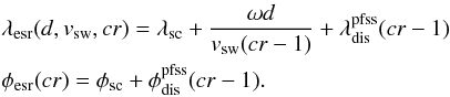 (8)The overall result for this method calculates to:
  (9)The results for the individual CRs are shown in Fig. 9 as green x. This is a more satisfying result than the two derived before. But if we look at the individual CRs in Fig. 9 there is a notable degree of variation, ranging from 75% of the source regions captured, for example, CR2055, down to only around 30%, for example, CR2050. To understand this variation we compared the mentioned examples with their respective preceding CR which was used to determine λesr(d,vsw,cr) and φesr(cr). This is done in Fig. 11.
 |
Fig. 11 Comparison between consecutive CRs. The left panels show the solar wind velocity taken from ACE for the respective CRs while the right panels show the PFSS model data of the photospheric foot points of the open magnetic field line. The latter rotations 2055 and 2050 are shown in red, the former rotations 2054 and 2049 are shown in blue. The upper panels show the case for CR 2055, where the predictions produced very good results while the lower panel show the case for rotation 2050, where only very poor results were produced. |
It is evident that the differences between CR 2054 and 2055 are rather small, hence the specific deviation method was able to produce such good results. The opposite is true for the rotations 2050 and 2049. Here the differences are considerable. Therefore it is only reasonable that the hit percentage is very low for CR 2050 and high for rotation 2047. From Figs. 11 and 9 it can be inferred that the correct prediction of the source regions depends critically one the similarity between consecutive CRs. If the similarities are not sufficient, the predictions made become unreliable.
In the case of SPICE constantly imagining the source regions for every step in Solar Orbiter’s orbit the method to specifically predict the source regions could be considered a satisfactory method since it leads to many cases where the source regions are successfully captured. SPICE will also be used for different purposes, therefore it will only image the solar wind’s source regions for certain selected points during its orbit. With only a small number of images the risk of not capturing even one source region becomes considerable. This renders the procedure discussed in this chapter rather unfavorable in the end. A different and more reliable method is discussed in the next section.
3.4. Leading stripe mapping
Instead of predicting each solar wind source region individually one could point the spectrograph at the sun with or without a certain leading angle while also trying to maximise the covered area on the Sun’s surface. Six observations per day can be vertically stacked in order to increase the instruments field of view. This increased field of view has a height of 96 arcmin and completely covers the Sun in terms of latitude. In this section we analyze the feasibility of such an approach. Solar Orbiter’s orbit and the observation of solar wind is simulated in the same manner as before. For each point in its orbit SPICE takes an image of the Sun’s surface with a fixed leading angle λla, pointing at  (10)With this configuration SPICE is able to capture virtually any source region on the Sun’s surface, but not necessarily at the actual solar wind release time. For each CR we calculate the coordinates of the solar wind’s source position and for every source coordinate we also determine the solar wind release time tps. The orbit is then simulated as described above ten times for different leading angles λla ranging from − 50° to 40°. Due to the rotation of the Sun, source regions enter the projection of the field of view coming from lower longitudes. As soon as a source region is located in the center of SPICE’s field of view it counts as observed. For each observed source region the remote observation time tobs is listed. Due to the rotation of the Sun the source region enters the field of view on the left side, that is, at lower longitudes. The field of view then sweeps over the source region until it is no longer covered. A source region stays roughly between 40 and 90 h inside the field of view, depending on the leading angle. In order to analyze this simulation we calculate the time difference between the release time of the solar wind package tps and the observation time tobs for every source region:
  (11)The results are shown in Fig. 12.
 |
Fig. 12 Results for the leading stripe mapping. The x axis shows the time difference Δt = tps − tobs between the time when a source region is observed by the spectrograph and when it releases its solar wind package. The y axis shows the probability per bin. The red curves show only source regions with a measured solar wind speed below 350 km s-1, the green curves represent intermediate speeds from 350 km s-1 to 600 km s-1 and the blue curves with speeds above 600 km s-1. Each panel shows the result for a different leading angle. The dashed vertical lines mark the area where a source regions would be observed at the moment of the solar wind’s release. The colored numbers show Γoc in percent with the corresponding errors. The errors are the statistical errors originating from the variation between individual CRs. |
Each panel shows the results for a different leading angle, starting with the upper left panel at λla = − 50° and ending with the lower right panel at λla = 40°. The histograms are normalized to their respective sum. The y axis therefore gives the probability per bin. The differently colored histograms show source regions with measured solar wind speeds below 350 km s-1, only source regions with speeds above 600 km s-1, and intermediate speeds with 350 km s-1<vsw< 600 km s-1. On the x axis Δt is shown. A negative value for Δt means that a particular source region has been observed by SPICE after the solar wind package was released, a positive value means the source region has been observed before the solar wind package departed. The area taking the extent of the field of view into account is marked. As stated above, a source region needs 40 to 90 h to traverse the field of view. With SPICE’s intention to observe a source region during the release of the solar wind, the area between the dashed lines marks the optimal observation time. We call the portion of source regions which are optimally covered Γoc.
If we now analyze the shown distributions of Δt it is evident that it shifts from right to left with increasing leading angle. With a leading angle of λla = − 50° the majority of solar wind packages are observed before the release of the solar wind package. Then again, a leading angle of λla = 30° and greater means the observation of nearly all source regions happens after the solar wind is released. We note that the difference between fast and slow solar wind is small. On the one hand the ballistic displacement leads to a systematic separation between the distributions of the fast and slow solar wind, since it depends on the solar wind speed. The magnetic displacement on the other hand does not depend on vsw and therefore leads to a broadening of both distributions and therefore to a distinctive overlap.
Since SPICE’s goal is to find the source regions of the slow solar wind we will focus on the red histograms in Fig. 12. The optimal solution would be a leading angle which enables SPICE to observe the solar wind’s source region at the moment when the solar wind is released, that is, when Γoc becomes maximal. This is the case for a leading angle λla ≈ 0°, as can be seen in the respective panel in Fig. 12. To examine this in more detail we repeat the simulation for leading angles ranging from − 8° to 2°. The results are shown in Table 2.
Γoc for solar wind with speeds <350 km s-1, as function of the leading angle.
It can be seen that the best results are achieved for leading angles λla between − 6° and − 4°. For the study of fast and intermediate solar wind a leading angle of λla = 10° would be optimal.
The errors shown in Fig. 12 derive from the variation between the individual CRs. These statistical errors are considerably larger than the ones derived from the method described in Sect. 2.4, which are of the order of 0.5% and smaller. From that we conclude that the uncertainties from the ballistic and magnetic mapping play only a secondary role in comparison to the statistical error.
4. Comparison with the CSSS model
As stated in Sect. 2, the CSSS model has been shown to predict solar wind speed nearly twice better than the PFSS model. The details of the CSSS model and the method adopted for the prediction technique can be found in Poduval & Zhao (2014) and Poduval (2016). In order to test if a different input model alters the results of our analysis we repeated the analysis of the former section but using the CSSS model for the calculation of the magnetic mapping. Additionally we adjust the radius of the source surface to 15 R⊙, as this is the case for the CSSS model. Since we have only a smaller subset of CRs computed with the CSSS model we also used the same smaller subset of rotations computed with the PFSS model for the comparison. The results are shown in Fig. 13.
 |
Fig. 13 Comparison of the leading stripe mapping between the PFSS (red histograms) and the CSSS (blue histograms) model. The axes are the same as in Fig. 12. Note that the subset of CRs used for this comparison only includes four rotations. The solar wind speed window covers the range from 0 to 350 km s-1. The errors given are the statistical errors originating from the variation between the CRs. |
The histograms shown here cover the same solar wind speed window as the red histogram in Fig. 12. The differences from Fig. 12 are because of the smaller subset of CRs used. In Fig. 13 we can see that both results show the same behaviour. Although the absolute numbers differ slightly both histograms show that the optimal value for Γoc is obtained for λla = − 10°. This analysis shows that the CSSS results are comparable to those of the well-established PFSS model. Therefore, for the present analysis both the CSSS and PFSS models seem equally applicable.
5. Summary and conclusion
One of the aims of the upcoming Solar Orbiter mission is to directly identify the source regions of solar wind by linking remote and in situ observations. The novelty of Solar Orbiter’s instrumentation lies in the capability of measuring solar wind in situ and remotely at the same time and very close to the Sun. The challenge to establish the link is not only to find the spatial displacement between in situ observed solar wind and its source region on the Sun but also to take into account the temporal displacement between these two observations. This means that we need to point the remote-sensing instrument on the right place at the Sun and at the right time. In order to do so the terminal solar wind speed as well as the magnetic configuration inside the corona must be known. Both cannot be known in real time, for example, the terminal solar wind speed cannot be obtained from remote sensing but only by in situ measurements. Thus, a prediction of the solar wind speed which will be measured in situ in the future is needed to point the spectrograph at the right place at present.
In this study we investigated the spatial and temporal displacement between in situ observed solar wind and its source region on the Sun. In addition we tested different methods to predict the optimal pointing of SPICE with respect to source region coverage and temporal displacement. The spatial displacement is found by tracking the solar wind from its source region out to the spacecraft. Above the source surface we applied classic ballistic back mapping, resulting in a ballistic displacement. Inside the corona we applied a PFSS model which yields a magnetic displacement, and a model by Cranmer et al. (2007) from which we derive the coronal escape time.
We find that it is important to consider the magnetic mapping in addition to the ballistic mapping for the prediction of the solar wind’s source regions. For the prediction of the solar wind’s release time, that is, the time when the instrument has to do its observation, the plasma escape time has to be added to the ballistic travel time of the plasma package. For an instrument to track the source regions in real time, a prediction scheme that uses the solar wind speeds and magnetic configuration of the preceding CR yields a probability of 45.56 ± 15.77% to observe the source region at the time of the solar wind’s release at the photosphere.
SPICE will only be able to make one raster per day, that is, SPICE will not be able to track the source regions at all times, but the in situ instrument (HIS) will measure at all time. To account for this a leading stripe forward mapping was devised, where six snapshots are vertically stacked to form a stripe which covers the whole Sun in latitude. Virtually any source region will be detected eventually, but typically not at the time of the plasma release at the Sun. For each source region covered by the leading stripe the time difference between remote observation and solar wind release can be calculated. To optimize the number of observations done at the right time the leading angle of the stripe can be varied. We tested this for various angles ranging from − 50° to 40° and three different solar wind speed regimes. This results in an optimal leading angle ≈− 6° for the study of slow solar wind (250 km s-1<vsw< 350 km s-1), ≈20° for intermediate (350 km s-1<vsw< 600 km s-1) and ≈10° for fast solar wind (600 km s-1<vsw< 900 km s-1).
Additionally we repeated the leading stripe method while using CSSS maps for the magnetic mapping in order to compare the results. The comparison did not lead to different results, hence we concluded that the PFSS model is sufficient for the presented analysis. In particular these small leading angles and the corresponding almost optimal line of sights are advantageous for the quality of the SPICE measurements. Although the focus of our study was on the upcoming Solar Orbiter mission and the SPectral Imaging of the Coronal Environment instrument, the methods described are generally applicable.
Acknowledgments
This work uses magnetograms obtained from the MDI instrument in board the SOHO spacecraft, SOHO is a project of international cooperation between ESA and NASA. Additionally this work uses SOLIS data obtained by the NSO Integrated Synoptic Program (NISP), managed by the National Solar Observatory, which is operated by the Association of Universities for Research in Astronomy (AURA), Inc. under a cooperative agreement with the National Science Foundation. The authors would like to thank Dr Bala Poduval for her valuable support with the CSSS model and the computations contributed to this work. R.f.W.S. acknowledges constructive discussions with the Solar Orbiter SPICE steering committee and the Solar Orbiter Science Working Team and the German Space Agency, DLR for grant 50OT1202. L.B. was supported by DLR grant 50OC1501.
References
- Altschuler, M. D., & Newkirk, G. 1969, Sol. Phys., 9, 131 [Google Scholar]
- Bochsler, P. 2000, Rev. Geophys., 38, 247 [NASA ADS] [CrossRef] [Google Scholar]
- Caldwell, M. 2014, SPICE Instrument User Manual [Google Scholar]
- Cranmer, S. R., van Ballegooijen, A. A., & Edgar, R. J. 2007, ApJS, 171, 520 [Google Scholar]
- Fisk, L. A. 2003, J. Geophys. Res. (Space Physics), 108, 1157 [Google Scholar]
- Fludra, A., Griffin, D., Caldwell, M., et al. 2013, in Solar Physics and Space Weather Instrumentation V, Proc. SPIE, 8862, 88620F [CrossRef] [Google Scholar]
- Geiss, J., Gloeckler, G., & von Steiger, R. 1995, Space Sci. Rev., 72, 49 [Google Scholar]
- Goel, A., & Choudhuri, A. R. 2009, Res. Astron. Astrophys., 9, 115 [NASA ADS] [CrossRef] [Google Scholar]
- Hassler, D. M., Deforest, C., & Spice Team 2011, AGU Fall Meeting Abstracts [Google Scholar]
- Koskela, J. S., Virtanen, I. I., & Mursula, K. 2015, AGU Fall Meeting Abstracts [Google Scholar]
- Krieger, A. S., Timothy, A. F., & Roelof, E. C. 1973, Sol. Phys., 29, 505 [NASA ADS] [CrossRef] [Google Scholar]
- Landi, E., Gruesbeck, J. R., Lepri, S. T., & Zurbuchen, T. H. 2012, ApJ, 750, 159 [Google Scholar]
- Liu, Y., & Norton, A. 2001, Mdi measurement errors: the magnetic perspective, SOI technical note, Tech. Rep., Stanford University [Google Scholar]
- Neugebauer, M., Forsyth, R. J., Galvin, A. B., et al. 1998, J. Geophys. Res., 103, 14587 [NASA ADS] [CrossRef] [Google Scholar]
- Nolte, J. T., & Roelof, E. C. 1973, Sol. Phys., 33, 241 [Google Scholar]
- Poduval, B. 2016, ApJ, 827, L6 [NASA ADS] [CrossRef] [Google Scholar]
- Poduval, B., & Zhao, X. P. 2014, ApJ, 782, L22 [NASA ADS] [CrossRef] [Google Scholar]
- Rappazzo, A. F., Matthaeus, W. H., Ruffolo, D., Servidio, S., & Velli, M. 2012, ApJ, 758, L14 [NASA ADS] [CrossRef] [Google Scholar]
- Royal Observatory of Belgium, B. 2016, http://sidc.be/silso/home [Google Scholar]
- Schatten, K. H., Wilcox, J. M., & Ness, N. F. 1969, Sol. Phys., 6, 442 [Google Scholar]
- Scherrer, P. H., Bogart, R. S., Bush, R. I., et al. 1995, Sol. Phys., 162, 129 [Google Scholar]
- Schwenn, R., Mohlhauser, K. H., & Rosenbauer, H. 1981, in Solar Wind 4, ed. H. Rosenbauer, 118 [Google Scholar]
All Tables
Terminal velocities and travel times from transition region to source surface for different flux tube models.
All Figures
|
Fig. 1 Displacement between the spacecraft’s coordinates and the source region’s coordinates. The magnetic connection of a fast (blue) and slow (red) solar wind package are shown in the reference frame of the spacecraft. The bending of the field lines below the source surface causes the magnetic displacement, the rotation of the Sun during the travel time from the source surface to the spacecraft causes the ballistic displacement. A solar wind package starts at the time tps at the photosphere, reaches the source surface at tss and is measured at tsc by the spacecraft. The colored dashed lines indicate the magnetic connection between spacecraft and the solar wind’s sources. |
| In the text | |
|
Fig. 2 Magnetic field map to illustrate the PFSS mapping. The intersection points with the source surface and foot points of the open magnetic field lines of the PFSS model are shown in red and green, where the colors depict the inward and outward polarities. The determined source-field lines and their course through the corona are shown in blue. The PFSS map corresponds to CR 2050, the underlying magnetogram is based on MDI observations. |
| In the text | |
|
Fig. 3 Sunspot number as a function of time. The blue curve gives the actual sunspot number and the red curve the monthly average. The variation in the Sun’s activity cycle is easily visible. The green shaded area marks the sequence of CRs we used for this study. The blue and red shaded areas mark sequences of CRs we investigated for comparison, the blue one also happens during the quiet time of the Sun while the red one happens during the active Sun. Data taken from Royal Observatory of Belgium (2016). |
| In the text | |
|
Fig. 4 Magnetic induced longitudinal (left) and latitudinal (right) displacement between source surface position and photospheric position. The y axis gives the number of occurrences for both plots normalized for the maximum. The calculation was made for an equatorial spacecraft path over the course of 19 consecutive CRs, each plot also shows a fit with a simple Gaussian (left) or a sum of two Gaussian (right). The fit parameters are given in the respective panels. The arrow marks δλ. |
| In the text | |
|
Fig. 5 Magnetic displacement for the other two time periods in Fig. 3 in the same manner as in Fig. 4. The period from 1881 until 1899 took place during the quiet phase of the Sun, but the magnetograms are from the Kitt Peak Observatory. The period from 1964 until 1982 took place during the active phase of the Sun where the PFSS model is not reliable. |
| In the text | |
|
Fig. 6 Investigated orbit of Solar Orbiter shown in orange. The x and the y axes define the ecliptic plane, the z axis is perpendicular to the ecliptic. The units for the axes are AU. The full Solar Orbiter orbit is shown in red, the orbit of Earth is shown in blue, the Sun is shown as yellow circle. The upper panel also contains the orbits of Mercury and Venus as additional reference points. We note that the z axis in the lower panel has a different scale from the y axis. Hence the out-of-ecliptic extent of the orbit seems exaggerated. |
| In the text | |
|
Fig. 7 Solar wind speeds used for this study. The solar wind speeds have been measured by ACE/SWEPAM during CRs 2040 to 2058. |
| In the text | |
|
Fig. 8 Projection of a field of view on the Sun. The left panel shows Solar Orbiter (dark red point) in orbit around the Sun (black mesh) with SPICE’s rectangular field of view (red) projected onto different regions of the Sun’s surface (not to scale). The right panel shows the projection on the Sun’s surface in heliographic coordinates. This is the actual projection of SPICE’s field of view from 0.3 AU, hence the right panel is to scale. |
| In the text | |
|
Fig. 9 Percentage of hits H(cr) plotted against the CR. The different colors depict the different methods used. The dashed lines represent the average of H(cr) for each method. The individual error bars stem from the error estimation described in Sect. 2.4. |
| In the text | |
|
Fig. 10 PFSS induced longitudinal (left) and latitudinal (right) displacement between source surface position and photospheric position similar to Fig. 4. The y axis gives the normed number of occurrences for both plots. The calculation was made for Solar Orbiter’s orbit over the course of 19 consecutive CRs, each plot also shows a fit with a simple Gaussian (left) or rather a sum of two Gaussian (right). We note the stronger shift to lower latitudes compared to Fig. 4 due to Solar Orbiter’s tilted orbit. |
| In the text | |
|
Fig. 11 Comparison between consecutive CRs. The left panels show the solar wind velocity taken from ACE for the respective CRs while the right panels show the PFSS model data of the photospheric foot points of the open magnetic field line. The latter rotations 2055 and 2050 are shown in red, the former rotations 2054 and 2049 are shown in blue. The upper panels show the case for CR 2055, where the predictions produced very good results while the lower panel show the case for rotation 2050, where only very poor results were produced. |
| In the text | |
|
Fig. 12 Results for the leading stripe mapping. The x axis shows the time difference Δt = tps − tobs between the time when a source region is observed by the spectrograph and when it releases its solar wind package. The y axis shows the probability per bin. The red curves show only source regions with a measured solar wind speed below 350 km s-1, the green curves represent intermediate speeds from 350 km s-1 to 600 km s-1 and the blue curves with speeds above 600 km s-1. Each panel shows the result for a different leading angle. The dashed vertical lines mark the area where a source regions would be observed at the moment of the solar wind’s release. The colored numbers show Γoc in percent with the corresponding errors. The errors are the statistical errors originating from the variation between individual CRs. |
| In the text | |
|
Fig. 13 Comparison of the leading stripe mapping between the PFSS (red histograms) and the CSSS (blue histograms) model. The axes are the same as in Fig. 12. Note that the subset of CRs used for this comparison only includes four rotations. The solar wind speed window covers the range from 0 to 350 km s-1. The errors given are the statistical errors originating from the variation between the CRs. |
| In the text | |
Current usage metrics show cumulative count of Article Views (full-text article views including HTML views, PDF and ePub downloads, according to the available data) and Abstracts Views on Vision4Press platform.
Data correspond to usage on the plateform after 2015. The current usage metrics is available 48-96 hours after online publication and is updated daily on week days.
Initial download of the metrics may take a while.