| Issue |
A&A
Volume 665, September 2022
|
|
|---|---|---|
| Article Number | A108 | |
| Number of page(s) | 29 | |
| Section | Galactic structure, stellar clusters and populations | |
| DOI | https://doi.org/10.1051/0004-6361/202244112 | |
| Published online | 15 September 2022 | |
The Gaia-ESO survey: A spectroscopic study of the young open cluster NGC 3293⋆,⋆⋆
1
Space sciences, Technologies and Astrophysics Research (STAR) Institute, Université de Liège, Quartier Agora, Allée du 6 Août 19c, Bât. B5c, B4000 Liège, Belgium
e-mail: [email protected]
2
Centre National d’Etudes Spatiales, Toulouse, France
3
Observatoire de Genève, Université de Genève, Chemin Pegasi 51, 1290 Versoix, Switzerland
4
Sorbonne Université CNRS, UMR 7095, Institut d’Astrophysique de Paris, 75014 Paris, France
5
Royal Observatory of Belgium, Ringlaan 3, 1180 Brussels, Belgium
6
Observatório Nacional/MCTIC, R. Gal. José Cristino 77, São Cristovão, 20921-400 Rio de Janeiro/RJ, Brazil
7
Institut für Astro- und Teilchenphysik, Universität Innsbruck, Technikerstr. 25/8, 6020 Innsbruck, Austria
8
Department of Physics and Astronomy, Notre Dame University-Louaize, PO Box 72 Zouk Mikaël, Lebanon
9
Department of Chemistry and Physics, Saint Mary’s College, Notre Dame, IN 46556, USA
10
Instituto de Astrofísica de Canarias, 38205 La Laguna, Tenerife, Spain
11
Universidad de La Laguna, Dept. Astrofísica, 38206 La Laguna, Tenerife, Spain
12
Institute of Astronomy, KU Leuven, Celestijnenlaan 200D, 3001 Leuven, Belgium
13
Institute of Theoretical Physics and Astronomy, Vilnius University, Sauletekio av. 3, 10257 Vilnius, Lithuania
14
Institute of Astronomy, University of Cambridge, Madingley Road, Cambridge CB3 0HA, UK
15
INAF – Osservatorio Astrofisico di Arcetri, Largo E. Fermi 5, 50125 Florence, Italy
16
INAF – Osservatorio Astronomico di Palermo, Piazza del Parlamento 1, 90134 Palermo, Italy
17
Max-Planck Institut für Astronomie, Königstuhl 17, 69117 Heidelberg, Germany
18
Niels Bohr International Academy, Niels Bohr Institute, University of Copenhagen Blegdamsvej 17, 2100 Copenhagen, Denmark
19
INAF – Padova Observatory, Vicolo dell’Osservatorio 5, 35122 Padova, Italy
20
Instituto de Astrofísica de Andalucía-CSIC, Apdo. 3004, 18080 Granada, Spain
21
Space Science Data Center – Agenzia Spaziale Italiana, via del Politecnico, s.n.c., 00133 Roma, Italy
22
Dipartimento di Fisica e Astronomia, Università di Padova, Vicolo dell’Osservatorio 3, 35122 Padova, Italy
Received:
25
May
2022
Accepted:
19
July
2022
We present a spectroscopic analysis of the GIRAFFE and UVES data collected by the Gaia-ESO survey for the young open cluster NGC 3293. Archive spectra from the same instruments obtained in the framework of the ‘VLT-FLAMES survey of massive stars’ are also analysed. Atmospheric parameters, non-local thermodynamic equilibrium (LTE) chemical abundances for six elements (He, C, N, Ne, Mg, and Si), or variability information are reported for a total of about 160 B stars spanning a wide range in terms of spectral types (B1 to B9.5) and rotation rate (up to 350 km s−1). Our analysis leads to about a five-fold increase in the number of cluster members with an abundance determination and it characterises the late B-star population in detail for the first time. We take advantage of the multi-epoch observations on various timescales and a temporal baseline, sometimes spanning ∼15 years, to detect several binary systems or intrinsically line-profile variables. A deconvolution algorithm is used to infer the current, true (deprojected) rotational velocity distribution. We find a broad, Gaussian-like distribution peaking around 200–250 km s−1. Although some stars populate the high-velocity tail, most stars in the cluster appear to rotate far from critical. We discuss the chemical properties of the cluster, including the low occurrence of abundance peculiarities in the late B stars and the paucity of objects showing CN-cycle burning products at their surface. We argue that the former result can largely be explained by the inhibition of diffusion effects because of fast rotation, while the latter is generally in accord with the predictions of single-star evolutionary models under the assumption of a wide range of initial spin rates at the onset of main-sequence evolution. However, we find some evidence for a less efficient mixing in two quite rapidly rotating stars that are among the most massive objects in our sample. Finally, we obtain a cluster age of ∼20 Myr through a detailed, star-to-star correction of our results for the effect of stellar rotation (e.g., gravity darkening). This is significantly older than previous estimates from turn-off fitting that fully relied on classical, non-rotating isochrones.
Key words: open clusters and associations: individual: NGC 3293 / stars: fundamental parameters / stars: abundances
Full Tables 1, 4, and 5 are only available at the CDS via anonymous ftp to cdsarc.u-strasbg.fr (130.79.128.5) or via http://cdsarc.u-strasbg.fr/viz-bin/cat/J/A+A/665/A108
© T. Morel et al. 2022
 Open Access article, published by EDP Sciences, under the terms of the Creative Commons Attribution License (https://creativecommons.org/licenses/by/4.0), which permits unrestricted use, distribution, and reproduction in any medium, provided the original work is properly cited.
This article is published in open access under the Subscribe-to-Open model. Subscribe to A&A to support open access publication.
1. Introduction
Young open clusters have long been recognised as key testbeds for our understanding of the physics and evolution of massive stars because they provide a snapshot of a stellar population sharing the same distance and initial chemical composition, but with members that span a very wide mass range. The cluster NGC 3293 (also known as the Gem Nebula) belongs to the small cohort of not too distant, well-populated ensembles of massive stars that are particularly well suited for that purpose. The cluster lies in the north-western outskirts of the Carina Nebula (NGC 3372), which is one of the most interesting and intense sites of star formation relatively nearby (Smith & Brooks 2008). Its distance, which was recently estimated to be 2.3–2.4 kpc based on Gaia EDR3 astrometric data, is fully compatible with that of the Carina association to which it is thus likely physically associated (Göppl & Preibisch 2022). Although it is not expected to host any O stars owing to its moderate age (∼10–15 Myr; e.g., Baume et al. 2003; Preibisch et al. 2017; Bisht et al. 2021), it is actually one of the most populous stellar aggregates in the Carina Nebula region (e.g., Preibisch et al. 2017). It contains tens of relatively unevolved early B stars (Evans et al. 2005), along with a few blue and red supergiants, including HD 91969 (B0 Ib) and V361 Car (M1.5 Iab), for instance. It also hosts some objects of particular interest, such as a chemically peculiar, strongly magnetic B2 star (CPD −57°3509; Przybilla et al. 2016) or several multiperiodic β Cep pulsating variables, among which one in an eclipsing binary (HD 92024; Engelbrecht & Balona 1986).
The Gaia-ESO public survey (hereafter GES) is a recently completed, ambitious spectroscopic survey of ∼105 stars in the Milky Way. The two main components of the project consist in observations of the field population and open clusters. As discussed by Bragaglia et al. (2022), NGC 3293 was selected as one of the young southern clusters to be intensively observed as part of the survey. The observations are made with the multi-object instrument Fibre Large Array Multi-Element Spectrograph (FLAMES; Pasquini et al. 2002) installed on the Very Large Telescope (VLT), enabling the simultaneous observation of the fields with the GIRAFFE and UVES spectrographs. The main aim of the GES is to supplement the Gaia space mission (Gaia Collaboration 2016) in order to address several issues related to the formation and evolution of the Milky Way (Gilmore et al. 2022; Randich et al. 2022). Complementary ground-based observations are particularly advantageous when studying massive stars because Gaia offers less diagnostic power for stellar characterisation, especially in terms of abundances. A discussion of the stellar parameters recently released as part of Gaia DR3 can be found in Fouesneau et al. (2022) and Blomme et al. (2022a). The former study includes a comparison with the GES results for OB stars where a large dispersion is usually observed1.
NGC 3293 has a long history of photometric measurements (e.g., Feinstein & Marraco 1980; Baume et al. 2003; Bisht et al. 2021), but spectroscopic investigations are much less common. Pioneering studies of this kind include Feast (1958), who obtained radial velocities (RVs) and spectral classification for the brightest stars, and Balona (1975) who determined their projected rotational velocities. Most abundance studies in the literature are restricted to the brightest cluster members (Mathys et al. 2002; Niemczura et al. 2009a). However, this cluster was also chosen by the GES because it was studied in some detail by the large ESO programme ‘VLT-FLAMES survey of massive stars’ (hereafter FS; Evans et al. 2005)2. As such, it can be used for benchmarking.
We take advantage of the largest spectroscopic dataset gathered to date for NGC 3293 to study the properties of its stellar B-type population in terms of spectral variability, chemical abundances, and rotational velocities. The age of the cluster is also revisited thanks to a thorough correction of our results for the effects of fast rotation. The FS led to the determination of fundamental stellar parameters and abundances for a sizeable number of early B-type stars. Our study can be regarded as being complementary to that of the FS and a leap forward towards a comprehensive characterisation of this cluster. In particular, we extend the determination of homogeneous parameters and chemical abundances to much lower masses (down to B9.5). Our study also brings about a number of improvements. For instance, to increase the sample size, the conclusions drawn by the FS about the rotational and chemical properties of this cluster (Dufton et al. 2006; Hunter et al. 2009) were based on the combination of the results with those of two other Galactic clusters, NGC 4755 and NGC 6611, even though the latter is much younger. In contrast, our results are entirely based on a statistically sound sample of stars whose membership to NGC 3293 can be established on a firmer footing thanks to the recently available Gaia data. For these various reasons, we revisit the results obtained by the FS. In addition, we reanalyse their GIRAFFE and UVES spectra for completeness and validation purposes.
This paper is structured as follows. Section 2 clarifies how our work fits into the context of the GES. Section 3 discusses the selection of targets and their membership, while Sect. 4 presents the observations. Our results concerning the atmospheric parameters, variability and binarity, and chemical abundances are provided in Sect. 5. Section 6 is devoted to a discussion of the rotational velocity distribution and age of the cluster after accounting for the effects of rapid rotation. Our main findings about the chemical properties of our targets are presented in Sect. 7. Finally, our main conclusions are given in Sect. 8.
2. This work in the context of the GES
The GES consortium is divided into several working groups (WGs). WG13 is in charge of the analysis of the OBA stars (Blomme 2011; Blomme et al. 2022b). As other WGs in the GES consortium, a number of research groups (called ‘nodes’) within WG13 independently analysed the spectra using their own techniques and codes. Following a critical evaluation of the quality of the data products from each node, the individual results are weighted and eventually combined to produce recommended, homogenised parameters and abundances. An important point is that, unlike the case of the cool stars treated by the other WGs, the abundances are not computed adopting the recommended parameters. Instead, to ensure self-consistency, the abundance determination performed by each node is based on its own set of atmospheric parameters. Full details about the scientific objectives, data collected for young clusters, organisation, and data processing procedures implemented in WG13 can be found in Blomme et al. (2022b).
The present paper presents the results obtained for NGC 3293 by the ‘Liège node’ based on the final data release of the survey (iDR6). Preliminary results based on iDR3 have been discussed by Semaan et al. (2015). As a cautionary note, our results slightly differ from those to be delivered by the GES to ESO for subsequent archiving and public release to the community because of the homogenisation phase described above. The comparison is discussed in Appendix A where it is shown that the differences are minor, except for the projected rotational velocity because of a quite poor agreement between the various nodes (Blomme et al. 2022b; see also Sect. E.2.2). The main purpose of the complex GES homogenisation procedures is to ensure optimal consistency across the various WGs, minimise systematics with respect to similar ongoing or forthcoming spectroscopic surveys, and facilitate the global interpretation of the catalogue. The ultimate objective being to fulfil the top-level goals of the survey, which are deciphering the formation history and evolution of the various populations (thin and thick discs, bulge, and halo) making up our Galaxy. In contrast, all the results discussed in this paper are not recalibrated in any way and – more importantly – are obtained in a much more homogeneous and self-consistent way. As such, they are more suitable for a dedicated study of NGC 3293. For this particular cluster, it can be noted that the Liège node provided a significant fraction of all the parameters delivered by WG13, was assigned the highest weight during the homogenisation phase (1.50 compared to 0.58–0.81 for the other nodes that analysed this cluster), and is the only one providing abundance data (see Blomme et al. 2022b). This paper is the first of a series of WG13 publications presenting the analysis of the GES data collected for young open clusters.
3. Target selection and cluster membership
Starting with the list of stars observed by the GES in the field of NGC 3293 (Sect. 3.1), we first selected those suitable for a spectral analysis (Sect. 3.2) and finally identified in this sample clear non cluster-members (Sect. 3.3).
3.1. Initial selection of GES targets in the cluster
The pre-selection of the cluster members was performed by the GES prior to the first release of the Gaia data and solely relied on photometric criteria (see Bragaglia et al. 2022). The 2MASS catalogue was the main starting point. High-quality observations3 were first selected from the full dataset in a large area of 12.5′ radius (corresponding to the FLAMES field of view) around the cluster centre quoted in the WEBDA database4. High-quality, near-infrared (IR) data in all three bands (JHKs) were required for a star to be included in this large pool of candidates. This list was next cross correlated with various optical catalogues available in the literature (Delgado et al. 2011; Baume et al. 2003; Dias et al. 2006; Netopil et al. 2007; Evans et al. 2005). They provide detailed photometry, as well as membership information. The cross-match with the catalogue of Delgado et al. (2011) is straightforward, as it already lists 2MASS cross IDs. For the others, a positional match within 1″ was required. A star was considered further if at least one of the optical catalogues classifies it as a member, whereas it was excluded if it is identified as an interloper in all catalogues in which it is listed.
The apparent cluster radius is ∼6–7′ corresponding to a physical radius of ∼5 pc (Bisht et al. 2021; Preibisch et al. 2017). To mitigate contamination, only stars within a radius of 4.1′ (Baume et al. 2003) were initially kept. A number of stars studied by the FS (Evans et al. 2005) without any membership information from the optical catalogues are located much farther away (up to ∼10′) than the generally accepted radius. Whether the cluster is more spatially extended than commonly believed deserves further investigation, but it was decided to add them back in. In addition, less secure members were also observed to avoid having some FLAMES fibres not being allocated, which increases the proportion of contaminants (see Sect. 3.3).
To refine the selection, two dereddened colour-magnitude diagrams (CMDs) were used: J0 vs. (J − H)0 and V0 vs. (B − V)0. A pre-Gaia distance modulus of 12.2 mag (Baume et al. 2003), E(B − V) = 0.263 mag as quoted in WEBDA, and a canonical extinction law with RV = 3.1 (Cardelli et al. 1989) were assumed. Stars were kept if they fulfilled the following criteria:
and
3.2. Stars selected for spectral analysis
We determine the parameters and chemical abundances of stars covering the full Teff range of B stars, that is from 10 to 32 kK. The stars to be processed at the lower Teff boundary were selected by a visual inspection of the blend formed by Ti IIλ4468.5 and He Iλ4471.5: the Ti II feature dominates for A stars. After selection of the B-type spectra, we have at this stage data for 186 stars.
As a next step, we screened out spectra that are too noisy to be analysed or suffer from severe instrumental problems (i.e. a picket-fence pattern in the case of UVES). Finally, after visual inspection, we discarded objects displaying obvious spectral peculiarities, either a composite morphology pointing to a spectroscopic binary (SBn, with n ≥ 2) or a strong, double-peaked emission profile in Balmer lines that could safely be attributed to a massive circumstellar disc. Continuum emission from the disc in Be stars requires a specific treatment (e.g., Ahmed & Sigut 2017). However, the incidence of this type of objects is discussed in Sect. 6.2.
Single-lined (SB1) and tentative double-lined (SB2) binaries were treated further under the assumption that the secondary does not significantly bias our results through, for instance, continuum dilution. We find that the abundance distributions for the stars identified as single and SB1’s are indistinguishable.
As to whether parameters are provided in the presence of line-profile variations (LPVs) depends on the strength of the LPVs and sampling of the observations. The variations arise from pulsations or, in the late B stars, from rotational modulation of a spotted photosphere that is presumably a common phenomenon in this Teff regime (Balona 2019). Stars with strongly distorted line profiles were dropped unless the changes are reasonably well sampled (see example in Appendix B). Because our results rely on the co-addition of all (RV corrected) exposures, they may be regarded in this case as representative of the mean values averaged over the variability cycle. In contrast, stars with nearly symmetric profiles were kept irrespective of the number of observations.
3.3. Check of cluster membership based on Gaia EDR3 data
There are efforts within the consortium to assign cluster membership probabilities from Gaia astrometric data supplemented by GES RVs (Jackson et al. 2020, 2022). However, NGC 3293 was not considered because the analysis relies on GIRAFFE HR15N spectra that are not available. Furthermore, there are too few objects with a measured RV for the methods to be suitable.
Carrying out a full statistical modelling of the 3D kinematics is beyond the scope of this paper. However, we decided to examine the astrometric properties of our sample because the fraction of contaminants is anticipated to be quite high (Bragaglia et al. 2022). In particular, the cluster lies in a crowded region very close to the Galactic plane (b ∼ 0.07°). We first cross-matched the GES and Gaia EDR3 (Gaia Collaboration 2021) catalogues using a search radius of 2″. Duplicate entries in Gaia EDR3 were found in a few cases, but a spurious association can safely be rejected thanks to a mismatch in coordinate, parallax, or G magnitude. The parallax, ϖ, is well determined, with on average ϖ/σϖ ∼ 20–25. Because the quality of the Gaia data does not afford in that case to confidently assess membership, we conservatively kept stars with possible issues with the processing of the astrometric measurements or an ill-behaved solution: either a duplicated_source flag raised or a renormalised unit weight error, RUWE, above 1.4 (e.g., Lindegren 2020). The number of visibility periods, visibility_periods_used, is always sufficient (i.e. above 8; see Arenou et al. 2018).
The Gaia EDR3 parallaxes are affected by small zero-point biases, which are a complex function of the stellar brightness and colour, for instance. We applied corrections on a star-to-star basis following Lindegren et al. (2021a). Although the offsets are small (∼ − 33 μas on average for the sub-sample with reliable astrometric solutions), they are significant at the distance of the cluster and lead to a more peaked parallax distribution (Fig. 1). It supports the reliability and usefulness of these corrections for bright, blue sources.
 |
Fig. 1. Breakdown of the parallaxes for the stars with well-behaved astrometric solutions before (top panel) and after (bottom panel) applying the zero-point offsets of Lindegren et al. (2021a). A foreground star (GES 10344563–5813091) with a much larger parallax is off scale. The dashed lines show the mean values, while the dotted lines indicate the 3-σ thresholds. |
The astrometric data are shown in Fig. 2. A total of 16 likely foreground or background late B stars were identified by their parallax deviating by more than 3σ from the mean of the distribution that is found to be ⟨ϖ⟩ = 0.423 ± 0.021 mas after iterative 3-σ clipping for the sub-sample with well-behaved astrometric solutions. Although results are provided, they are not considered further when discussing the properties of the cluster (Sects. 6 and 7). GES 10343562–5815459 was retained because its parallax is only slightly above the threshold, while its proper motion is fully compatible with that of the cluster.
 |
Fig. 2. Astrometric and photometric properties of our sample. Red symbols highlight in all panels stars assumed not to be cluster members, while dark blue symbols indicate stars with possible issues with the Gaia EDR3 data. Left panels: proper motions. A typical error bar with a size multiplied by ten is shown. Top middle panel: parallax distribution. The dashed line shows our mean value. Bottom middle panel: coordinates (epoch J2000). Right panel: CMD. |
One can clearly notice in Fig. 2 (left panels) a group of nine presumed members with a right parallax, but large μα and low μδ values5. These stars are preferentially located to the north of NGC 3293 and therefore at the very northern edge of the Carina complex. They also have RVs that often differ from the cluster systemic velocity (Sect. 5.3). Although most of them probably belong to the field despite the fact that they lie at the right distance, they are all kept because a few could be runaways. We note that these nine stars (among which two eventually do not have parameters determined) would contribute to a level of contamination not exceeding ∼10%. Considering them in the following does not modify our conclusions in any appreciable way.
We end up with 149 stars for which we provide parameters (among which 141 have abundances). To this total, 16 stars with a variability or binarity flag can be added, which leads to a total of 165 objects with information of some sort. If only the members are counted, 137 and 130 stars have parameters and abundances, respectively. We estimate that about 120–130 B stars were identified by Baume et al. (2003) in the inner region (4.1′ circle radius) of the cluster through optical photometry. However, it only gives a very rough idea of our completeness level because the area we cover is much wider (Sect. 3.1).
4. Observational data
The GIRAFFE (R ∼ 20 000) and UVES (R ∼ 47 000) GES settings used are described in Blomme et al. (2022b). Only the UVES U520 blue arm was considered here because much more information is encoded compared to the red arm. Data were also obtained with the GIRAFFE HR09B grating, but are not used either because of the lack of useful diagnostic lines in the B-star regime. The bulk of the data were obtained during the period February–April 2012 (i.e. prior to GIRAFFE upgrade), while a few UVES spectra were acquired in January 2013. The HR04 grating was considered at a much later stage of the project in order to use Hγ as an additional surface gravity indicator (Berlanas et al. 2017). As a result, fewer stars have this setting available. The data were secured in December 2017. A small fraction of the GIRAFFE spectra (not HR04) appeared to be contaminated by that of a calibration lamp in the adjacent MEDUSA fibre. Depending on the severity of the problem, these spectra were either ignored or the associated results were given a lower weight.
For the FS data, HR05A and HR14A are replaced by HR05B and HR14B, respectively. The last two gratings have a better spectral resolution at the expense of a slightly narrower wavelength range (see Blomme et al. 2022b). The GIRAFFE data were supplemented by a few UVES spectra not discussed in Evans et al. (2005). All the raw FS data were retrieved from the ESO archives and pre-processed using exactly the same reduction procedures as for the GES data (Sacco et al. 2014; Gilmore et al. 2022). The FS HR02 data were not treated because they cover a wavelength region bluewards of any GES settings. We also draw attention to the fact that the GES ignored the FS observations of the brightest stars in the cluster (down to V ∼ 6.5) acquired with FEROS. Therefore, those data are not included in the present analysis.
Multi-epoch observations (secured ∼3 weeks apart) are often available for HR05A, while data for other settings may have been obtained during different nights. The availability of repeated observations (quite often up to four or five) allows us to carry out, to our knowledge, the first modern binary detection programme through spectroscopy since Feast (1958). In particular, the FS data were obtained over a single night. We take advantage of these data acquired much earlier (14 April 2003; Evans et al. 2005) to extend the time span of the observations to a baseline (9–14 years) appropriate for the detection of binaries with relatively long periods. The observations are described in Table 1. A timescale relevant to binarity was assumed to define the epochs: they are separated by more than one day. Observations secured on an hourly timescale that is commensurate with, for instance, pulsations were only obtained with UVES (see example in Appendix B). The breakdown of the number of independent epochs, total time span of the observations, and time interval between consecutive epochs is shown in Fig. 3. The histogram of the time span is dominated by three peaks: one corresponding to the two GES HR05A observations gathered ∼25 days apart, as well as two at large values arising from the late acquisition of the GES HR04 data and objects with both FS and GES spectra. Despite a time sampling that appears in principle suitable for the detection of binaries with a quite wide range of orbital periods (see bottom panel of Fig. 3), it is important to bear in mind that the cadence strongly varies across the sample. In addition, the RV time series were obtained with a variety of instrumental configurations.
 |
Fig. 3. Time sampling. Breakdown of number of independent epochs, Nb (top panel), total time span of observations, ΔT (middle panel), and time interval between consecutive epochs, δT (bottom panel). |
Summary of observations and sampling properties.
The mean signal-to-noise ratio (S/N) of the epoch spectra is shown for each setting in Fig. 4. The wide range of values reflects the fact that all stars in a single FLAMES pointing were observed with the same exposure time. As a result, the data quality for the faintest targets (i.e. late B-type dwarfs) is much lower. The S/N of the HR05A spectra eventually used for the parameter determination is generally better by a factor ∼1.4 because it is often the combination of two epoch spectra (Sect. 5.2). HR14A is not used for that purpose, but only for inferring the Si II and Ne I abundances. For the limited number of stars for which either of the two can be measured, the S/N lies in the range 55–490 with a mean of ∼180. For the stars with FS data reprocessed, we find that the quality of the corresponding GES HR06 spectra is similar. However, the S/N of the GES spectra is larger by a factor ranging from ∼1.1 (HR03) to ∼1.5 (HR04) for the other GIRAFFE gratings.
 |
Fig. 4. Breakdown of the mean S/N of the epoch spectra. The S/N is computed by the GES and refers to the value averaged across the entire wavelength range. The histogram for U520 is multiplied by five for better visibility. |
Finally, a number of benchmark OBA stars were observed during the survey (Pancino et al. 2017; Blomme et al. 2022b). To evaluate the reliability of our results, we analysed the high-quality data of 134 Tau (B9 IV), HD 56613 (B8 V), HD 35912 (B2 V), γ Peg (B2 IV), τ Sco (B0.2 V), and θ Car (B0 Vp). Regrettably, no HR04 spectra were obtained for this sample.
5. Analysis and results
Following a pre-processing of their spectra (Sect. 5.1), the objects eventually selected after filtering (Sect. 3) had their stellar parameters (Sect. 5.2), variability status (Sect. 5.3), and chemical abundances (Sect. 5.4) determined.
5.1. Data pre-processing
All reduction steps (e.g., extraction of the spectra from the CCD chip, wavelength calibration) are performed by WG7 prior to delivery of the spectra to WG13. No nebular correction was applied to the NGC 3293 data. The GES internally produces stacks of all the spectra obtained for a given target and instrumental setting over the whole survey (see Sacco et al. 2014). We extracted all the individual exposures and grouped them into epoch spectra: consecutive exposures were co-added and time-resolved spectra obtained over more than one day were treated separately.
By default, the spectra are normalised to the continuum by the GES reduction pipeline. However, this automatic procedure is optimised for cool stars and appears to lead to unsatisfactory results (line wings truncated) for the broad features (e.g., Balmer and helium lines) present in the spectra of OBA stars (Blomme et al. 2013). All spectra were therefore normalised manually using low-order polynomials with the IRAF6 software.
5.2. Determination of atmospheric parameters
We used global least-square minimisation to derive the stellar parameters. Using a Python code we developed, we fit the observed normalised spectra with a grid of solar-metallicity, synthetic spectra computed with the SYNSPEC48 program, along with local thermodynamic equilibrium (LTE) ATLAS97 (Kurucz 1993) and non-LTE TLUSTY8 (Lanz & Hubeny 2007) model atmospheres. The ATLAS9 and TLUSTY grids were employed for the stars with Teff below and above 15 kK, respectively. In both cases, a microturbulence, ξ = 2 km s−1, was used. Our analysis relies on codes assuming plane-parallel atmospheres in hydrostatic equilibrium. It is a suitable assumption given that none of our targets is expected to have a very strong wind. As a consequence, we do not provide any wind parameters, such as the mass-loss rate.
The first step consists in determining the RV and projected rotational velocity, V sin i, for all epoch spectra. The synthetic spectra are thus convolved with a rotational profile (Gray 2005), and then shifted in velocity. Instrumental broadening is taken into account. We did not consider broadening by macroturbulence, but it is expected to be largely dominated by rotation in our relatively unevolved targets (Simón-Díaz et al. 2017). Furthermore, as shown below, most of them are (very) fast rotators. We calculate the χ2 for each synthetic spectra and interpolate the χ2 map to determine the best-fitting values. As a next step, we corrected each epoch spectrum for its individual RV and combined all GIRAFFE settings of a given target into a single spectrum put in the laboratory rest frame. For the same target, FS and GES spectra were treated separately. Finally, the determination of Teff and log g is performed over the whole wavelength domain. The synthetic spectra are convolved with the rotational velocity averaged over the values obtained for each epoch settings and the combined spectra. Some examples of fits are shown in Appendix C. After determining Teff and log g, we used them to calculate anew the RV and V sin i of the individual epoch settings.
An uncertainty9 is associated to each measurement on the basis of the χ2 surface (1-σ contour). The typical random uncertainties are ∼800 K for Teff, ∼0.12 dex for log g, ∼11 km s−1 for V sin i and ∼3 km s−1 for RV. However, these figures considerably vary from star to star depending on the stellar parameters and data quality. As an illustration, V sin i and its uncertainty grow in parallel according to a typical ratio of about 5–6%.
5.3. Variability and binarity analysis
We emphasise that our approach to investigate the variability and binarity fundamentally differs from that adopted in the recent literature (e.g., Sana et al. 2013) in that we do not attempt to infer a robust binary fraction. It is because of the limitations affecting the GES observations that were not designed for this particular purpose and, above all, of the subjectivity in our pre-selection (Sect. 3.2) that can hardly be quantified. It is likely that the low binary occurrence rate we infer (∼15%) is grossly underestimated. Therefore, we refrain from discussing to what extent our (lower limit to the) binary fraction in NGC 3293 compares with that for B-type stars in other clusters (e.g., Dunstall et al. 2015; Banyard et al. 2022). Similarly to the approach followed by other studies (e.g., Holgado et al. 2018), our less ambitious goal here is instead to primarily flag stars whose determination of stellar parameters could potentially be affected by their spectral variability. As a byproduct, secure binary candidates are nonetheless identified.
The individual RVs produced at the end of the processing described in Sect. 5.2 were analysed to identify variable stars. The HR06 data were not used because the RVs are more uncertain and it would introduce some heterogeneity given that fewer objects were observed with this setting. The steps described in the following can also be regarded as some kind of validation of the RV measurements.
5.3.1. Confronting HR03 and HR04 settings
An important fraction of the targets were observed with both the HR03 and HR04 settings. For each object, we matched them by the pair of measured RVs. In case of three observations, we made two pairs with the isolated exposure being repeated. To avoid strong redundancy, in the case of two HR03 and two HR04 exposures, we formed only two pairs, taking care to match together the exposures most separated in time. The error in the RV difference within a pair, σd, is given by the quadratic sum of the RV uncertainties. If the individual standard deviations are correctly estimated, the normalised difference should indeed be a normal variate. We listed 136 pairs of RVs including 67 with exposures acquired on the same day. The last cases are interesting because they are not supposed to be markedly different from zero and are thus a good check that allows us to validate the differences in RVs.
The left panel of Fig. 5 illustrates the distribution of the normalised (by the expected error) differences corresponding to each pairs. It is seen that their probability density function (PDF) is rather clearly Gaussian with μ = 0 and σ = 1. The mean is actually slightly biased to μ = +0.4, but this is not to be considered as significant. It is interesting to notice that the 67 contemporaneous pairs are pretty well in agreement with the Gaussian curve. The errors in RV(HR03) and RV(HR04) are statistically similar. Thus σ = 1 is a good validation of the typical values for the errors in the individual RVs.
 |
Fig. 5. Histograms of the normalised difference RV(HR03)–RV(HR04) (left panel) and RV(HR03)–RV(HR05) (right panel) for all the pairs. All the objects are included in the black histograms. The green histograms only include the contemporaneous pairs. The red continuous lines represent a Gaussian PDF of zero mean, μ, and with either unit variance (left panel) or σ = 1.414 (right panel). GES 10352851–5812496 is off scale in the right panel. |
Some rarer objects present discrepant pairs and can be suspected of variability. Discrepant pairs go up to −14.6σ on one side and up to +8.0σ on the other side. Not knowing if the +0.4 offset affecting μ is real or not, we cautiously considered as candidate variables the pairs that are located outside of the ± 2.5-σ domain; we spotted out 20 pairs that are discrepant and retained for further investigation. They correspond to 15 different objects.
5.3.2. Confronting HR03 and HR05 settings
The same kind of approach can be applied to the RV difference HR03 vs HR05, where the HR05 dataset includes both HR05A and HR05B. We listed 274 pairs among which 159 are acquired on the same day. The distribution of the central part of the PDF is well Gaussian and centred on μ = 0 (right panel of Fig. 5). However, the dispersion is much larger with respect to the left panel leading to σ = 1.414. This is somewhat surprising since the standard deviation for HR05 is larger than for HR03 and HR04: this is taken into account, but the value could hardly be further increased. Thus the distribution should be narrower. The problem is probably due to a rather bad estimation of the RV uncertainties determined from HR05 for an unknown reason. Pairs are here also present in the tails of the distribution between −16.8σ and +19.0σ, except for GES 10352851–5812496, which is at 68.8σ. We thought reasonable to extend a little the threshold separating constant stars from variable candidates. A 4.0-σ criterion is producing 25 pairs related to potentially variable candidates that are retained for further inquiry. They correspond to 19 different objects. We did not investigate the pair of setting HR04 vs. HR05 to avoid redundancy.
5.3.3. Confronting identical settings
Finally, we built pairs of observations acquired with the same setting, at different epochs. We drew a list of seven discrepant pairs for HR03, four for HR04 and, finally, 16 for HR05A/B for which we have some suspicion of variability at the 3.0-σ level. As usual, all these selected pairs were retained for further analysis.
5.3.4. Confronting UVES spectra
In addition to the GIRAFFE spectra, we inspected a total of 69 FS and GES U520 spectra. They cover a wider wavelength domain encompassing many more lines. From a statistical point of view, treating them in a similar way as the GIRAFFE spectra is much more difficult. This UVES set contains 24 objects, among which eight have only UVES spectra. The 16 remaining ones have both UVES and GIRAFFE spectra in various proportion.
Out of the eight objects, two only have one FS spectrum available. One of these two clearly exhibits numerous examples of line doubling pointing to a probable SB2 character; while the other one has a peculiar spectral morphology (double-peaked emission lines). Four objects exhibit variability well beyond the 3-σ threshold; one is located at a more marginal level, but is confirmed variable by a detailed eye inspection. One object must be considered as constant. Finally, one has all its exposures severely affected by instrumental or reduction problems.
The situation is much more complex for the 16 objects that have both types of data (UVES + GIRAFFE) where the classification is a mix of the work described in the preceding sub-sections, that performed in case only UVES spectra are available, and detailed eye inspection. Including the star discussed above, it resulted in the total detection of seven constant objects observed with UVES. The others are suspected variables.
5.3.5. Flagging the variability and the binarity
Stars with changes in RVs that could be assigned to binary motion and/or a variable line shape were identified. The main criterion is an outlying value with respect to the distribution of the RV differences between pairs of GIRAFFE settings, namely, HR03 vs. HR04 and HR03 vs. HR05A/B. As a second step, objects presenting variations in the epoch spectra of a given setting were sought. In all cases, the relevant spectra were visually examined. Stars presenting significant variability on the basis of at least two criteria (i.e. between pairs of settings or for the same wavelength domain) are classified as true variables with a good significance level. An additional visual inspection helps to discriminate between SB1 (or previously unrecognised SB2) and intrinsic line-profile variables (due to pulsations or any other cause). The decision for objects with both UVES and GIRAFFE data is first based on the GIRAFFE spectra and is then aided by the information extracted from the UVES spectra. Among the stars clearly identified as binaries (confidence level ‘A’ or ‘B’), only GES 10361791–5814296 (secure SB1 and tentative SB2) has an anomalously high Gaia EDR3 RUWE indicating an ill-behaved astrometric solution with respect to the expectations for a single source.
The detailed results of the variability analysis are given in Table D.1. All the cases listed above are documented according to a flagging scheme (Van der Swaelmen et al. 2018; Gilmore et al. 2022). Although the flags specific to the WG13 Liège node (see Table 2) were provided on a star-to-star basis as part of the final public data release, we caution that they are superseded by those given here that rely on a more in-depth analysis. We also note that, because of the limited number of observations and inadequate time sampling over relatively short timescales, the flag reporting LPVs is often solely raised on the basis of profiles that are deemed to be asymmetric. Therefore, the identification of these variables is often not fully secure, especially in the cooler objects with fewer lines and a poorer S/N. Furthermore, the distinction between those and SB2’s is generally ambiguous. For these reasons, the status of the intrinsically variable and SB2 candidates requires confirmation.
Flags specific to the WG13 Liège node.
We count 113 objects (including 104 members) not listed in Table D.1 for which a lack of variations has been noticed with the data at hand. The breakdown of the mean RVs is shown in Fig. 6. The systemic velocity of the cluster is in agreement with previous estimates: for instance, from the FS (Evans et al. 2005) or Gaia DR2 (Soubiran et al. 2018).
 |
Fig. 6. Distribution of the mean RVs for the stars considered as constant. The red histogram is for stars assumed not to be cluster members, while the orange one is for the presumed members with the right parallax, but a discrepant proper motion (Sect. 3.3). The other stars are shown in black. The mean values found by Evans et al. (2005) and Soubiran et al. (2018) are shown as dashed and dotted lines, respectively. |
5.4. Determination of chemical abundances
The following chemical species were considered for the abundance analysis: He, C, N, Ne, Mg, and Si (both Si II and Si III). The non-LTE abundances were derived from a spectral synthesis of He Iλ4471, C IIλ4267, N IIλ4630, Ne Iλ6402, Mg IIλ4481, Si IIλ6371, and Si IIIλ4568-4575. Some illustrative fits are shown in Appendix A of Blomme et al. (2022b). These features were selected because they are relatively unblended and can be measured in the largest number of stars, even in case of a high rotation rate. Despite the much wider wavelength coverage of the UVES spectra, the same diagnostic lines were used to ensure consistency.
The non-LTE code DETAIL-SURFACE (Giddings 1981; Butler & Giddings 1985) coupled to Kurucz LTE model atmospheres was used for the line modelling. See Przybilla et al. (2011) for a justification of such a hybrid method for stars for which wind effects can be neglected. The model atoms are described in Morel et al. (2006) and Morel & Butler (2008). Synthetic C IIλ4267 profiles were computed with the carbon model atom developed by Nieva & Przybilla (2008). The line is not affected in NGC 3293 by nebular emission. Our carbon abundances are expected to be more reliable than those of the FS that were based on a more simplistic model ion and eventually corrected for a Teff trend (Hunter et al. 2009). Metal lines blended with the diagnostic features (e.g., Al IIIλ4480) were modelled assuming abundances typical of B-type stars determined with the same code (see Table 6 of Morel et al. 2008). Oxygen abundances for all stars and carbon abundances for those with Teff < 17 kK are not reported because of suspiciously large values or unexpected trends with some stellar parameters.
Given our inability to constrain the microturbulence, either from global fitting (Sect. 5.2) or from the analysis of individual lines, it was fixed to sensible values. Because late B dwarfs largely dominate our sample, ξ = 2 km s−1 was adopted for the synthetic DETAIL-SURFACE grids. However, except for the carbon grid that was built for another purpose, this quantity for the relatively evolved, early B stars (Teff > 22 kK and log g < 3.7 dex) was set to 5 km s−1. The dependence as a function of the stellar parameters is based on previous determinations in the literature (e.g., Hunter et al. 2009; Lefever et al. 2010; Lyubimkov et al. 2013; Nieva & Przybilla 2012).
The abundance uncertainties were empirically estimated by comparing the results for stars having multiple determinations from GES and archival data. For the stars with Teff > 20 kK, we also compared the abundances obtained for ξ = 2 and 5 km s−1 to take the impact of the choice of the microturbulence into account. The various sources of error were added in quadrature. Figure 7 shows the internal dispersion in the Mg abundances as a function of Teff and V sin i. In this particular case, irrespective of the V sin i, an uncertainty of 0.15 and 0.20 dex was assigned to stars cooler and hotter than 20 kK, respectively. For the other elements, no clear dependence with the parameters was found (as illustrated in Fig. 7 for He) and a single value was adopted. The 1-σ uncertainties lie in the range 0.1–0.3 dex for the metals and are fixed to 0.015 by number for helium10 (see Table 3), but were arbitrarily inflated by a factor 1.5 when the fit of the line was poor or the spectrum contaminated by that of a calibration lamp.
 |
Fig. 7. Variations of the dispersion in the Mg and He abundances (colour coded) as a function of Teff and V sin i. |
Nominal abundance uncertainties in dex (except y: by number).
5.5. Validation and final results
Through the analysis of repeated observations, we conclude that there is an overall satisfactory level of agreement between our parameters and abundances irrespective of the instrumental set-up (see Sect. E.1). We therefore assume that these are independent measurements and weight them by their random uncertainties to obtain the final, mean values provided in Table 4. A detailed comparison with respect to external sources (reference values for a set of benchmarks, results from other WG13 nodes or the FS for the stars in common) is provided in Sect. E.2.
Final parameters and abundances.
continued.
continued.
6. Discussion of apparent fundamental parameters and their parent non-rotating counterparts
Given that most targets are fast rotators, it is relevant to consider the influence of rotation on the observed stellar properties. For instance, stellar rotation can lead to a blurring of the main-sequence turn-off and mimic an age spread in young and intermediate age open clusters (e.g., Marino et al. 2018; Bastian et al. 2018). There is therefore a need to distinguish the physical quantities that are based on stellar model atmospheres and evolutionary tracks neglecting or not rotation.
6.1. Methodology
The first stellar quantities are called ‘apparent’ parameters and have been the subject of the previous sections. Those resulting from the use of models where the effects induced by the stellar rotation are taken into account are called ‘parent non-rotating counterparts’ (hereafter pnrc; Frémat et al. 2005; Zorec et al. 2016; Cochetti et al. 2020) and represent the objects as if they were at rest. These parameters for the sub-sample of 137 cluster members with spectroscopic parameters are discussed below. We consider as apparent quantities Teff, log geff, V sin i, as well as the bolometric luminosity, L. The last quantity is obtained from the apparent bolometric magnitude, Mbol, which is in turn obtained from the absolute magnitude in the V band, MV, following

where MV is calculated thanks to the Gaia EDR3 parallaxes and (G, GBP, GRP) photometric data (Gaia Collaboration 2021; Lindegren et al. 2021b). The Gaia parallaxes were corrected following Sect. 3.3, while the magnitudes were transformed into the Johnson-Cousins UBV system using the relations of Riello et al. (2021). We call also ‘apparent’ the stellar mass, M, and age, t, when they are obtained from the apparent Teff, log geff, and L through evolutionary models without rotation.
The intrinsic UBV colours are needed to estimate MV and the interstellar colour excess, E(B − V). They were interpolated as a function of the apparent parameters (Teff, log geff) in the tables of Castelli & Kurucz (2003), which were updated in 2011. We obtain ⟨E(B − V)⟩ = 0.29 ± 0.11 mag. The individual values given in Table 5 show quite a large spread. The patchy nature of the extinction has long been known (e.g., Turner et al. 1980) and arises from dust clouds obscuring part of this young cluster (Preibisch et al. 2017). The bolometric correction, BC(Teff), is taken from LTE model atmospheres (Castelli & Kurucz 2003) for Teff ≲ 15 kK and from non-LTE ones (Hubeny & Lanz 1995; Lanz & Hubeny 2007) when Teff ≳ 15 kK according to the recommendations of Pedersen et al. (2020). The (unavoidable) slight inconsistencies at the Teff boundary do not lead to appreciable errors. In both cases, the warnings put forward by Torres (2010) were taken into account.
Colour excesses and stellar parameters (pnrc, averaged over the stellar surface, and apparent).
continued.
continued.
The set of fundamental parameters corrected for effects carried by rotation is made of the pnrc Teff, pnrc(M, t), geff, pnrc(M, t), and Lpnrc(M, t). The quantity V(M, t)sin i is corrected for the overestimation discussed by Stoeckley (1968) induced by gravity darkening (GD; von Zeipel 1924; Espinosa Lara & Rieutord 2011). The actual stellar mass M, the age t of the star as a rotating object, and the inclination angle i of the rotation axis are considered pnrc, as opposed to those derived from the set of apparent (Teff, log geff, L) parameters and stellar models without rotation. All mentioned pnrc parameters and the V sin i corrected from GD effect are derived solving the following system of four equations:
![$$ \begin{aligned} {\left\{ \begin{array}{ll} \displaystyle P_\mathrm{app} = \displaystyle P_\mathrm{pnrc} (M,t)\ C_\mathrm{P} (M,t,\eta ,i) \\ \displaystyle \frac{(V\!\sin i)_\mathrm{app} }{V_\mathrm{c} (M,t)}\! =\! \displaystyle \left[\frac{\eta }{R_\mathrm{e} (M,t,\eta )/R_\mathrm{c} (M,t)}\right]^{1/2}\!\!\!\!\sin i-\frac{\Sigma (M,t,\eta ,i)}{V_\mathrm{c} (M,t)}, \end{array}\right.} \end{aligned} $$](/articles/aa/full_html/2022/09/aa44112-22/aa44112-22-eq5.gif)
where P ≡ Teff, log g, or L. The variables Papp and Ppnrc stand for the apparent and pnrc stellar parameters, while Vc is the critical velocity. The present-day, actual and critical stellar equatorial radii, Re(M/M⊙, t/tMS, η) and Rc(M/M⊙, t/tMS), are determined using 2D models of rigidly rotating stars (Zorec et al. 2011; Zorec & Royer 2012). The quantity, η = (Ω/Ωc)2[Re/Rc]3, is the ratio of the centrifugal to the gravitational acceleration at the equator where Ω is the surface angular velocity. On the right-hand side of Eq. (4), the functions CP(M, t, η, i) carry all the information relative to the change of parameters due to the oblateness of the rotating star and the concomitant GD effect over the observed hemisphere (Frémat et al. 2005; Zorec et al. 2016). The term Σ(M/M⊙, t/tMS, η, i) is Stoeckley’s correction that takes GD into account (Espinosa Lara & Rieutord 2011; Zorec et al. 2017). The current angular velocity is the result of the loss and redistribution of angular momentum undergone in the star since the pre-main-sequence phase. As no observational information exists about the internal angular velocity profile, the behaviour at the stellar surface, which is probably differential, is nevertheless taken here uniform over the whole area (rigid surface rotation). However, we adopt the time dependence, Ω ≡ Ω(t), as predicted by the Geneva evolutionary models with rotation (Meynet & Maeder 2000; Ekström et al. 2008, 2012; Georgy et al. 2013). A moderate core convective overshoot of 0.1Hp, where Hp is the local pressure scale height, is adopted for the relevant mass range (Ekström et al. 2012).
For each star, Eq. (4) is solved for 104 Monte Carlo trials. Each time, a new uncertainty, ϵP, corresponding to a given apparent parameter,  , is drawn at random according to a Gaussian distribution with a standard deviation given in Tables 4 and 5. Moreover, the system of equations must satisfy the condition that the V predicted by the model reproduces the observed V sin i corrected for GD. At each iteration step, the pnrc Teff and L that are input parameters to the evolutionary models with rotation are transformed into values averaged over the stellar surface deformed by rotation, so as to be similar in nature to the tabulated model quantities. The apparent and derived pnrc quantities are given in Table 5. We also provide the quantities averaged over the rotationally deformed stellar surface, log⟨Teff⟩, log⟨g⟩, and log(⟨L/L⊙⟩), that are best suited for a direct comparison with the model predictions. The Hertzsprung-Russell (HR) diagrams shown in Fig. 8 allow one to appreciate the impact of correcting for rotation-related effects. We note that using apparent stellar parameters leads to stars of the lower-main sequence lying significantly above the zero-age main sequence (ZAMS), which was a concern raised by Dufton et al. (2006) when analysing the FS data.
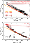 |
Fig. 8. HR diagrams using apparent (top panel) and averaged over the stellar surface (bottom panel) stellar parameters. Isochrones for various ages and initial rotation rates are overlaid (Georgy et al. 2013). |
Given the unknown incidence of magnetic stars in NGC 3293, specific models (e.g., Keszthelyi et al. 2019, 2020) are not discussed. Furthermore, only about 10% of all O and early B stars (Grunhut et al. 2017; Morel et al. 2015) or late B stars (Donati & Landstreet 2009) have a detected, large-scale magnetic field. Unlike the majority of our targets, they are usually (very) slow rotators because of magnetic braking or show some sort of chemical peculiarities, as illustrated by the case of CPD –57°3509 (Przybilla et al. 2016).
6.2. Rotational velocity distribution
The differences between the distributions of apparent and corrected surface rotational velocities, as obtained from the solutions of Eq. (4), are illustrated in Fig. 9. The distributions of the observed (apparent) V sin i are shown in the left panel, where the histogram corresponds to the raw values (Table 4). The class-steps of the histogram are established according to the bin-width optimisation method of Shimazaki & Shinomoto (2007). The smoothed version of the V sin i frequency density distribution corrected for measurement uncertainties, Ψ(V sin i), was calculated using kernel estimators (Bowman & Azzalini 1997). Each observed V sin i is represented by a Gaussian distribution, whose dispersion is given by the standard deviation of individual V sin i estimates. Also shown is the Φ(V) distribution of the apparent true velocities V, which was obtained using the Richardson-Lucy deconvolution method (Richardson 1972; Lucy 1974) under the assumption of a random distribution of viewing angles. The middle panel of Fig. 9 depicts the V sin i’s corrected for Stoeckley’s overestimation and the true velocities, Vpnrc, as they result from the solution of Eq. (4). Finally, the distributions of the ratios, (V sin i/Vc)pnrc, and true velocities, (V/Vc)pnrc, are shown in the right panel of Fig. 9. The error bars for the Ψ and Φ distributions are of similar magnitude. According to the distribution of the (V/Vc)pnrc ratios, most of the studied stars in the cluster have values in the range 0.2–0.8. The maximum of the histogram is at (V/Vc)pnrc ∼ 0.55, which translates into an equatorial acceleration ratio, η = 0.23. It is far from the critical ratio, η = 1.0. The transformation of (V/Vc)pnrc = 0.55 into a ratio of angular velocities leads to ωpnrc = 0.73, where ω = Ω/Ωc. It is also below the values closer to critical rotation commonly observed in Be stars.
 |
Fig. 9. Rotational velocity distributions. (a) Histogram (grey) and smoothed distribution (blue) of (V sin i)app. The Vapp distribution is shown in red; (b) same as left panel, but for rotational velocities corrected for GD; (c) histogram (grey) and smoothed distribution (blue) of velocity ratios corrected for GD, (V sin i/Vc)pnrc. The distribution of GD-corrected velocity ratios, (V/Vc)pnrc, is shown in red. |
The B stars lying on the high-velocity tail of the (V/Vc)pnrc distribution (i.e. with values above 0.7) are almost all of rather low mass, that is M ≲ 4–5 M⊙. They certainly need a very long time to display the Be phenomenon through the redistribution towards the surface of their internal angular momentum (Zorec et al. 2005). However, these stars could be considered members of the Bn class, which is an old terminology to designate rapidly rotating B stars and potential candidates to display the Be phenomenon (van Bever & Vanbeveren 1997; Baade & Rivinius 2000; Zorec et al. 2007). As shown in Fig. 10, most of the stars in the cluster have masses M ≲ 6 M⊙. While the maximum frequency of Be stars occurs for spectral type B2 (Zorec & Briot 1997), there is only 7% of stars with masses M/M⊙ ∼ 8.0 ± 2.1 and (V/Vc)pnrc ∼ 0.74 ± 0.15. This may partially explain that the number of classical Be stars is very low despite the fact that they are common in open clusters with an age in the range 13–25 Myr (Fabregat & Torrejón 2000). We only found five stars showing clear evidence for emission in Balmer lines (one shell-like), which is very similar to the tally already reported by the FS (Evans et al. 2005) or McSwain et al. (2009) despite our larger sample. A transition from an absorption to a strong double-peaked Hα emission profile is observed between the FS and GES observations of CPD −57°3531 (GES 10360595–5814270), confirming its strongly transient nature (McSwain et al. 2009). Although stars with stable discs are relatively straightforward to detect, even with snapshot observations, other transients might have evidently escaped detection. The seven probable Be stars lying in the outskirts of the cluster proposed by Baume et al. (2003) from narrow-band photometric indices were not observed by the GES. We do not expect any Herbig Ae/Be stars in our sample. Although star formation is still believed to be operating in NGC 3293, according to Baume et al. (2003) or Delgado et al. (2016) only lower-mass stars with spectral types later than about A5 may still be contracting on their way to the ZAMS.
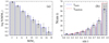 |
Fig. 10. Stellar mass and inclination angle distributions. (a) pnrc masses; (b) inclination angles compared to the theoretical distribution for values at random. |
The solution of Eq. (4) also provides the inclination angle of the stellar rotation axis whose sine distribution is compared with that for angles drawn at random in Fig. 10. On account of the uncertainties that plague the angle estimates, there is no indication in this cluster for significant deviations from a global isotropic distribution. The case of other clusters is discussed, for instance, by Jackson & Jeffries (2010).
6.3. Age of the cluster
From models of stellar evolution, it is apparent that the relationships for stars with masses M ≲ 6 M⊙ between evolutionary time and either L or Teff are near ‘vertical’ loci. It implies that the interpolation of ages for stars in this range of masses is highly sensitive to uncertainties in the above input parameters (i.e. to small deviations in ϵL or ϵTeff). In some extreme cases, it can lead to assign the objects to either the ZAMS or the terminal age main-sequence (TAMS). To avoid spurious estimates of ages, we impose two limitations to the values obtained from solving Eq. (4). Thus, the lowest accepted ages should represent an epoch after the nominal beginning of the ZAMS, which corresponds to the stabilisation phase of the initial angular momentum redistribution in the star (Meynet & Maeder 2000). To the opposite side of the age distribution, ensuring the consistency of all stellar fundamental parameters for the given rotational rate also acts to rule out extreme values. These limitations produce the truncated shape of the age histograms shown in Fig. 11. Four objects without trustworthy solutions were rejected. The lack of dependence between stellar mass and age ensures that the low-mass stars do not bias our estimate (see above). The fractional ages, t/tMS, derived from evolutionary models with rotation are smaller that those obtained from models neglecting it. Nevertheless, the time tMS that a rotating star spends on the main sequence is substantially longer compared to its non-rotating counterpart. For this reason, the mean cluster age, log(t) [yr] = 7.31 ± 0.26, is ∼10% larger than the value when rotation is not taken into account. The age uncertainty is not the standard deviation of the mean, but is computed based on the outcome of the Monte Carlo simulations (Sect. 6.1). As it takes all the sources of error thoroughly into account, it must be regarded as a rather conservative estimate.
 |
Fig. 11. Distribution of stellar ages derived from ‘apparent’ (red) and corrected for GD (blue) fundamental parameters. |
7. Discussion of abundance results
Before discussing the surface chemical properties of the cluster stars, we note that a self-consistent analysis would have required a (tedious) correction of our abundances for GD effects, as described in the previous section for the atmospheric parameters. According to Frémat et al. (2005), however, we anticipate that such changes would be small for the relevant rotation rates (see also Cazorla et al. 2017).
7.1. General abundance properties
Figure 12 shows the variations of the abundances as a function of the stellar parameters for both the cluster stars and the benchmarks. The data are compared to the mean values for NGC 3293 reported by the FS (Hunter et al. 2009) and the most recent set of solar abundances (Asplund et al. 2021). We find systematically larger average abundances than the FS (see also Fig. E.5). However, except for Si, our estimates for the metals still lie significantly below the solar values, as also found by Mathys et al. (2002) or Niemczura et al. (2009a). Yet there is no reason to believe that this young cluster is metal poor (Strobel 1991; Niemczura & Daszyńska-Daszkiewicz 2005). A mean LTE iron abundance fully consistent with solar was also reported by Trundle et al. (2007). The observed discrepancies might be remedied by the use of better model atoms (Nieva & Przybilla 2012), although we note that a state-of-the-art modelling was employed for C IIλ4267 (Nieva & Przybilla 2006, 2008).
 |
Fig. 12. Variations of the abundances as a function of the apparent stellar parameters. Non cluster-members (Sect. 3.3) were excluded. Stars with or without a binary flag are shown with open and filled symbols, respectively. Stars flagged or not as line-profile variables are plotted as squares and circles, respectively. For both variability types, a confidence level ‘A’ or ‘B’ is required. The benchmarks are shown with star symbols (for convenience, the position of those discussed in Sect. 7.3 is indicated in the panels showing the behaviour of the N and [N/C] abundances as a function of Teff). Crosses show illustrative error bars. The Si II and Si III data are plotted together in the same panels. The horizontal, dashed line indicates the solar abundance (Asplund et al. 2021), while the horizontal stripe shows the mean values (±1σ) for stars in NGC 3293 determined by Hunter et al. (2009). The values are provided in Table 6. The rightmost panels show the breakdown of our abundance data for the NGC 3293 sample. |
As a preamble to discussing the dependence between the chemical abundances and the stellar parameters, we recall that our sample spans an exceptionally wide Teff and V sin i range. As a consequence, our analysis is prone to systematic errors, for instance, because of Teff-dependent deficiencies in the modelling or biases in the treatment of the narrow-lined vs fast-rotating stars. It is therefore important to interpret the results cautiously. This danger is illustrated by the behaviour of helium. As can be seen in Fig. 12, we obtain supersolar He abundances and an increase as a function of Teff for the early B stars. We chose He Iλ4471 as our unique diagnostic because this strong, diffuse line can be measured in virtually all stars. However, as part of the GES iDR3 processing cycle, we experimented with He Iλ4713, which is intrinsically much weaker and cannot be measured in many objects. We found that the difference between the He Iλ4471- and He Iλ4713-based abundances increases as a function of Teff, and reaches up to Δy ∼ 0.04 at ∼25 kK. A similar tendency was noticed during our past abundance studies of nearby B-type stars also based on DETAIL-SURFACE (Morel et al. 2006, 2008). We conclude that relatively large line-to-line abundance differences may be expected and that the Teff trend is likely an artefact. A helium excess in the B0–B0.2 V stars τ Sco and θ Car is not supported by previous studies (e.g., Hubrig et al. 2008), and might instead be found in dwarfs more massive and rotating dramatically faster (e.g., Howarth & Smith 2001; Cazorla et al. 2017). We note that GES 10354901–5814541 (CPD −57°3509) that is known to be a strongly magnetic, He-rich star (Przybilla et al. 2016) was flagged as a line-profile variable and later discarded given the unsuitability of standard models.
There are only six stars with both Si II and Si III abundances. The mean difference shows a large scatter (−0.21 ± 0.40 dex; Si II minus Si III), as expected because of the large uncertainties affecting the abundances. On an individual basis, the largest (at the 2- to 3-σ level) discrepancies are found for the two early B stars where Si IIλ6371 begins to vanish and is barely measurable. Given the limited information at hand, it is unclear whether any meaningful conclusions about the Teff scale can be drawn from Si ionisation balance.
7.2. Chemically peculiar objects
Figure 13 shows the distributions for each abundance ratio of the residuals with respect to the mean value, which was estimated by iteratively removing any stars deviating by more than 3σ. The Si II-based abundances are ignored because they are only estimated for a handful of stars. The mean values for the whole sample are given in Table 6 and compared to previous estimates in the literature. The distributions of the residuals in Fig. 13 appear compatible with the measurement errors. It shows that the cluster is globally chemically homogeneous to within our level of precision.
 |
Fig. 13. Distributions for each abundance ratio of the residuals with respect to the mean values (Table 6). Non cluster-members (Sect. 3.3) were excluded. A normal distribution with a standard deviation corresponding to the mean of our final random uncertainties is overplotted with a dashed line. The two stars with peculiar abundances are indicated in red. |
Mean abundances for NGC 3293 compared to the solar photospheric values (Asplund et al. 2021) and previous non-LTE spectroscopic studies in the literature.
There are only two slowly rotating, quite evolved late B stars (GES 10355513–5811053 and GES 10362103–5810530) clearly at odds with the statement made above that the cluster is chemically homogeneous. This conclusion is primarily based on account of their very low Mg abundances, but they are He-poor as well (Fig. 13). Late B stars with a severe Mg depletion are discussed, for instance, by Hempel & Holweger (2003). There are no other abundances available and they are not identified as binaries. The weak decline of the Mg abundances for lower V sin i (Fig. 12) is remarkably similar to that observed in other late B-type samples (Niemczura et al. 2009b) and may be ascribed to mild diffusion effects in the slow rotators. It is unclear whether the lower abundances for hotter or more evolved objects is also of physical origin (for a possible correlation as a function of Teff, see Fossati et al. 2011), but empirically correcting for these trends does not erase the dependence with V sin i. The two peculiar stars fall about 0.5–1.0 dex below the values for stars with similar Teff or log g, which supports their classification as chemically peculiar.
The Hg IIλ3984 line, which is one of the prime diagnostics for a HgMn classification is not covered by our observations. However, a cursory inspection of the spectra allowed us to confidently detect several Mn II lines (at λ4137, λ4363, λ4365, and λ4479 Å) in GES 10355440–5812563 (FS 3293-064). This star was too cool to be processed with our code and was classified as A0 II by Evans et al. (2005). Identifying chemically peculiar stars in clusters with a precise age estimate is particularly valuable. However, its Gaia EDR3 data clearly identify it as a foreground object with a discrepant proper motion.
It is well known that radiative levitation and gravitational settling can lead in late B stars to surface abundances dramatically departing from solar (e.g., Hempel & Holweger 2003; Niemczura et al. 2009b). The high spin rates of our targets (Fig. 9) may inhibit the development of diffusion processes, although some chemically peculiar objects are unexpectedly quite fast rotators (e.g., González et al. 2021). As mentioned in Sect. 3.2, we only processed stars selected on the basis that Ti IIλ4468.5 is weaker than He Iλ4471.5. The pitfall of such a simple approach is that it may be biased against the selection of He-weak objects. Stars with peculiar spectra could also have been rejected because they were poorly fit with our synthetic spectra computed for a scaled-solar chemical composition. It would also contribute to the apparent lack of stars with strongly unusual surface abundances.
7.3. C and N abundances as proxies of internal mixing
Rotation triggers the transport of angular momentum and chemicals in stellar interiors. It notably leads to changes in the chemical abundances seen at the surface of massive stars and, in particular, a nitrogen excess accompanied by a lower-amplitude carbon depletion (e.g., Daflon et al. 2001). Observations by the FS have unveiled two unevolved stellar populations in the Magellanic Clouds that exhibit surface nitrogen abundances not predicted by single-star evolutionary models incorporating rotational mixing (Hunter et al. 2008, 2009; Brott et al. 2011): namely, slow rotators with an unexpected excess of nitrogen and, conversely, fast rotators with no or little nitrogen enrichment at their surface (see also, e.g., Rivero González et al. 2012; Grin et al. 2017; Dufton et al. 2020). The inability of evolutionary models to reproduce these two populations has been questioned (Maeder et al. 2009, 2014), but there are clear examples where they fail to reproduce the observations (e.g., Keszthelyi et al. 2021). The origin of these two populations is a matter of speculation, but might result from the action of magnetic fields (e.g., Keszthelyi et al. 2019) or mass-transfer processes in binaries (e.g., de Mink et al. 2013; Song et al. 2018; Mahy et al. 2020). However, although slowly rotating, N-rich B dwarfs have long been known in the field (Gies & Lambert 1992), they were not clearly detected in the Galactic clusters observed by the FS, including NGC 3293 (see Fig. 6 of Hunter et al. 2009).
As seen in Fig. 12, the dramatic nitrogen overabundance in the primary of the post-mass transfer binary θ Car is confirmed (Hubrig et al. 2008). If similar spun-up objects following an accretion event were present in our sample, it is very likely that they would have been detected, but none is found. We only discuss below the [N/C] abundance ratio because it is a more robust indicator of the dredge up of core-processed material at the surface of OB stars. First, because the evolutionary changes affecting C and N are inversely correlated. Second, because the C II- and N II-based abundances have the same qualitative sensitivity to errors in Teff, for instance. We adopt as baseline for this ratio our mean value, [N/C] ∼ −0.5, found for the two benchmarks γ Peg and HD 35912. They have both been shown from high-precision studies to have a [N/C] fully compatible with solar (Nieva & Simón-Díaz 2011; Nieva & Przybilla 2012). A few stars show some observational evidence for a modest N enhancement exceeding the 3-σ level. Two of them (GES 10355539–5812197 and GES 10360491–5810433) with [N/C] ∼ −0.1 are about boron normal and therefore very unlikely to have experienced deep mixing (Proffitt et al. 2016). The N-rich status of some of these candidates is therefore questionable. Nonetheless, we confirm earlier claims (e.g., Hunter et al. 2009) that the cluster lacks a population of strongly N-enriched stars. This conclusion is supported by the fact that an analogue of τ Sco that is known to show a relatively mild enhancement would be spotted quite easily. As shown in Fig. 12, we recover the well-known nitrogen overabundance of this star (e.g., Martins et al. 2012).
We now compare our [N/C] measurements to the expectations from solar-metallicity evolutionary models that incorporate the effects of rotation on the internal stellar structure (Georgy et al. 2013). The predicted abundance ratios were scaled such that the baseline value on the ZAMS is [N/C]ZAMS = −0.5 (see above). As discussed by Ekström et al. (2012), the default value of the models at the onset of main-sequence evolution is [N/C]ZAMS = −0.61 (Asplund et al. 2005). The stars with [N/C] data constitute a heterogeneous sample in terms of pnrc mass and ω values. A basic property of models of massive stars is that the amount of core-processed material dredged up to the surface strongly depends on the rotational velocity. To ensure a meaningful comparison, the wide range of ω values determined in Sect. 6 thus requires the use of a set of models matching the current stellar rotation rates. As a result, it is first necessary to associate for each star the current, observed ω to the appropriate value at birth (see, for instance, Ekström et al. 2008 for the evolution of ω along the evolution for the Geneva models). As shown in Fig. 14, the two quantities are roughly equivalent for the fiducial age of the cluster irrespective of the mass. For simplicity, we therefore assume in the following that the present-day ω is representative of the initial value on the ZAMS, ωinit.
 |
Fig. 14. Model dependence between the current ω and mass for log(t) = 7.3 (Georgy et al. 2013). The behaviour is shown for rotation rates at birth, ωinit, ranging from 0.1 to 0.95. The observed ω and M values for the stars with and without [N/C] data are overplotted as filled circles and open squares, respectively. For clarity, only the former are shown with error bars. The star GES 10355661–5812407 is off scale because of a spuriously large mass. |
The [N/C] data are compared in Fig. 15 to the theoretical values for various initial rotation rates and two cluster ages, log(t) = 7.2 and 7.4, that bracket our mean estimate. Accounting for the uncertainty in the cluster age, overall we do not detect outstanding, systematic discrepancies with respect to the model predictions. However, one exception is GES 10360160–5815096 (FS 3293-012 or V380 Car) for which [N/C] is much lower than expected. Our C abundance is large and quite uncertain, but other studies also reported a low [N/C] ratio (Hunter et al. 2009; Niemczura et al. 2009a). Furthermore, it is not at all boron depleted (Proffitt et al. 2016). A somewhat less convincing case for a similar behaviour is provided by GES 10354822–5812329 (FS 3293-019 or V405 Car), which is another confirmed β Cep star (Stankov & Handler 2005). A low [N/C] is once again confirmed (Hunter et al. 2009), but it is slightly boron depleted (Proffitt et al. 2016) contrary to V380 Car. These two stars are indicated in Fig. 15. It thus appears that a consistent picture is not entirely achieved under the assumption of a wide (possibly mass-dependent; Huang et al. 2010) distribution of spin rates at birth. It is in particular telling that the only noteworthy disagreement is found for two fast-rotating, massive stars (ω ∼ 0.44 and M/M⊙ ∼ 18 for V380 Car, while ω ∼ 0.64 and M/M⊙ ∼ 8 for V405 Car) that are among the most sensitive probes of rotational mixing in our sample. The others are either slow rotators or not massive enough.
 |
Fig. 15. Comparison in a HR diagram between the [N/C] data (squares) and the predictions (circles) of solar-metallicity evolutionary models for various initial rotation rates and two cluster ages: log(t) = 7.2 (left panels) and 7.4 (right panels). The model predictions are taken from Georgy et al. (2013). The stars selected in each panel fulfil the condition |ω − ωinit| < 0.1. The observational error bars are smaller than the square symbols. The [N/C] abundance ratio is colour coded. The stars V380 Car – and to a lesser extent V405 Car – whose observations are at odds with the model predictions are indicated. |
8. Summary and conclusions
We present a homogeneous analysis of the Galactic open cluster NGC 3293 based on GES and FS VLT-FLAMES observations of about 160 B-type member candidates spanning a wide range of physical properties. To our knowledge, it is the most comprehensive spectroscopic study of this cluster to date.
We infer the present-day intrinsic distribution of the rotational velocities for stars spanning the whole B1–B9.5 domain through a deconvolution algorithm. Our analysis supports the results from the FS (Dufton et al. 2006)11, and suggests for the full sample a Gaussian-like velocity distribution that peaks around 200–250 km s−1. We do not find evidence for a bimodal distribution as claimed, for instance, for the relatively unevolved, early B-type stars in 30 Doradus (Dufton et al. 2013). However, our sample does not contain enough B0–B3 stars to investigate the shape of the distribution for this particular population. Most stars in NGC 3293 appear to rotate at ∼50–60% of their critical velocity, as is also the case for other samples dominated by largely unevolved, late B-type stars (Huang et al. 2010). In contrast, however, significantly lower spin rates are observed for more massive members (Fig. 14). Similar mass-dependent distributions are observed in h & χ Per (Strom et al. 2005), which is a solar-metallicity open cluster of about the same age. The distribution for the O stars in the Carina nebula peaks at lower velocities (Berlanas et al., in prep.). Our results are not directly comparable, however, because it is a younger population in which spin-down effects due to stellar winds are much more important. A caveat resulting from the incompleteness of the binary census in NGC 3293 is the unknown importance of physical effects potentially experienced by close binaries, such as tides or mass-transfer processes (see, e.g., Ramírez-Agudelo et al. 2015; Mahy et al. 2020). Notwithstanding, a more fundamental difficulty is that post-interaction objects may be truly single (i.e. mergers) or go unnoticed through a standard RV monitoring (de Mink et al. 2014).
We obtain a cluster nuclear age of ∼20 Myr based on a realistic distribution of the spin rates and a detailed correction on a star-to-star basis for the effect of stellar rotation. It is larger than the typical value obtained from photometric studies that made use of non-rotating isochrones (∼10–15 Myr; e.g., Baume et al. 2003; Bisht et al. 2021): for instance, the Padova-Trieste suite of models (Girardi et al. 2000; Marigo et al. 2017) employed by the two papers cited above. However, there is a case in young clusters from a comparison with independent estimates from the lithium depletion boundary method for an underestimation of ages from isochrone fitting when the models do not take the full range of effects induced by rotation into account (Cummings & Kalirai 2018): namely, the combination of changes in the evolutionary paths and in the photometric properties because of GD. This raises the issue of a possible upwards revision of the age of young open clusters that host a large proportion of fast rotators, as has been invoked in older ones (e.g., Brandt & Huang 2015). Whether physical processes other than rotation significantly contribute to the spread observed near the turn-off of very young clusters is still debated (e.g., Li et al. 2019). But, in any case, rotating models (let alone because of their extended core hydrogen-burning lifetime) are an essential ingredient of any attempt to interpret the observational properties of an ensemble of fast-rotating massive stars (e.g., Meynet & Maeder 2000; Georgy et al. 2014). The extent of the apparent age spread in clusters spanning a very wide range of ages is well reproduced by rotating Geneva models (Georgy et al. 2019).
By quite a significant margin, NGC 3293 appears to be the oldest stellar aggregate in the Carina Nebula complex (see Preibisch et al. 2017). Although not observed by the GES, we note that the position of the red supergiant V361 Car (M1.5 Iab–Ic) in the HR diagram is also compatible with our inferred age when adopting the spectroscopic parameters of Arentsen et al. (2019). Its membership is confirmed by Gaia EDR3 data and the RV of Feast (1958). To the opposite side of the mass spectrum, the status of the O7 V((f))z star HD 91824 has for long been debated (e.g., Feinstein & Marraco 1980). Although its Gaia EDR3 proper motion is indistinguishable from that of the bona fide members, it is likely a foreground object based on its parallax that is discrepant at a level exceeding 5σ. It is a known SB1 (Sota et al. 2014), but its RUWE does not indicate problems with the astrometric solution. Unless it is a rejuvenated binary product, the existence of an unevolved O Vz star in such a moderate aged cluster is not expected (e.g., Arias et al. 2016).
Finally, this cluster appears to be to a large extent devoid of objects exposing core-processed material at their surface despite the fact that most of them are fast rotators. We argue it is primarily the consequence of most members being low-mass B dwarfs. Overall, the lack of widespread deviations from the baseline CN abundances (e.g., Fig. 13) is in agreement with the theoretical expectations for the cluster age once the rotation rate of the evolutionary model is matched to the observations. However, noteworthy exceptions are two quite rapidly rotating, apparently single sub-giants with little, if any, evidence for internal mixing (even shallow) based on their boron and nitrogen abundances. It suggests that the efficiency of rotational mixing is overestimated in these two objects. We note that our conclusion about the lack of strongly N-enriched stars in NGC 3293 extends to the more massive and evolved stars not observed by the GES. Only the two brightest B-type members classified as supergiants by Evans et al. (2005), whose membership is confirmed from Gaia EDR3, show some evidence for a mild N enrichment at similar levels as found in our sample (Hunter et al. 2009)12. Concerning the abundance properties in more general terms, macroscopic transport in (non magnetic) stars is known to inhibit the development of diffusion processes (e.g., Michaud et al. 2015 and Niemczura et al. 2009b for theoretical and observational arguments, respectively). Meridional circulation arising from fast rotation may thus largely account for the low occurrence of chemical peculiarities for helium and the metals not affected by evolutionary effects. From a completely different perspective, it might also explain the dearth of faint, high-order g-mode B pulsators, as speculated by Balona (1994).
Because the space velocities are of less importance here, we ignored the bias of the order of 40 μas yr−1 affecting the Gaia EDR3 proper motions for stars with G < 13 mag (Cantat-Gaudin & Brandt 2021).
Taken from POLLUX database available at http://npollux.lupm.univ-montp2.fr/
BSTAR2006 grid available at http://nova.astro.umd.edu/
We note that their estimate of the underlying rotational velocity distribution is also based on data for NGC 4755, which presumably has similar characteristics.
Two caveats can be noted: the FS Teff scale has been claimed to be too cool for early B-type stars (Proffitt et al. 2016) and the N abundance might be slightly revised following improvements in the data reduction (Dufton et al. 2018).
The only exception to the rule is GES 10361503–5808043 for which the V sin i based on GES data appears underestimated (210 vs 302 km s−1; Fig. E.1) from the inspection of the fit to the metal features used for the abundance analysis (Sect. 5.4). In addition, ROBGrid obtained 300 km s−1. All the GES results for this star are therefore ignored.
The ON node convolved their synthetic spectra assuming a macroturbulence fixed to 5 km s−1, but rotation largely dominates the line broadening for the seven stars in Fig. E.3.
Acknowledgments
We would like to thank the anonymous referee for useful comments that led to a clearer presentation of our results. T.M. acknowledges financial support from Belspo for contracts PRODEX Gaia-DPAC and PLATO mission development. He is grateful to Keith Butler for making the DETAIL-SURFACE code available to him. E.G. is grateful to Belgian F.R.S.-FNRS for multiple supports. A.B. and T.S. are thankful for grants of Concerted Research Actions (ARC) financed by the Federation Wallonie-Brussels. A.L. acknowledges funding received in part from the European Union Framework Programme for Research and Innovation Horizon 2020 (2014–2020) under the Marie Sklodowska-Curie grant Agreement No. 823734. M.F.N. acknowledges the support of the Austrian Science Fund (FWF) via a Lise-Meitner Fellowship under project number N-1868-NBL. L.M. thanks the European Space Agency (ESA) and the Belgian Federal Science Policy Office (Belspo) for their support in the framework of the PRODEX Programme. W.S. acknowledges FAPERJ for a Ph.D. fellowship. M.B. is supported through the Lise Meitner grant from the Max Planck Society. She acknowledges support by the Collaborative Research centre SFB 881 (projects A5, A10), Heidelberg University, of the Deutsche Forschungsgemeinschaft (DFG, German Research Foundation). This project has received funding from the European Research Council (ERC) under the European Union’s Horizon 2020 research and innovation programme (Grant agreement No. 949173). This paper is based on data products from observations made with ESO Telescopes at the La Silla Paranal Observatory under programme ID 188.B-3002. These data products have been processed by the Cambridge Astronomy Survey Unit (CASU) at the Institute of Astronomy, University of Cambridge, and by the FLAMES/UVES reduction team at INAF/Osservatorio Astrofisico di Arcetri. This work was partly supported by the European Union FP7 programme through ERC grant number 320360 and by the Leverhulme Trust through grant RPG-2012-541. We acknowledge the support from INAF and Ministero dell’Istruzione, dell’Università e della Ricerca (MIUR) in the form of the grant ‘Premiale VLT 2012’. The results presented here benefit from discussions held during the Gaia-ESO workshops and conferences supported by the ESF (European Science Foundation) through the GREAT Research Network Programme. This work has made use of data from the European Space Agency (ESA) mission Gaia (https://www.cosmos.esa.int/gaia), processed by the Gaia Data Processing and Analysis Consortium (DPAC, https://www.cosmos.esa.int/web/gaia/dpac/consortium). Funding for the DPAC has been provided by national institutions, in particular the institutions participating in the Gaia Multilateral Agreement. This research has made use of NASA’s Astrophysics Data System Bibliographic Services, the SIMBAD database operated at CDS, Strasbourg (France), and the WEBDA database, originally developed by Jean-Claude Mermilliod, and now operated at the Department of Theoretical Physics and Astrophysics of the Masaryk University.
References
- Ahmed, A., & Sigut, T. A. A. 2017, MNRAS, 471, 3398 [Google Scholar]
- Arenou, F., Luri, X., Babusiaux, C., et al. 2018, A&A, 616, A17 [NASA ADS] [CrossRef] [EDP Sciences] [Google Scholar]
- Arentsen, A., Prugniel, P., Gonneau, A., et al. 2019, A&A, 627, A138 [NASA ADS] [CrossRef] [EDP Sciences] [Google Scholar]
- Arias, J. I., Walborn, N. R., Simón Díaz, S., et al. 2016, AJ, 152, 31 [NASA ADS] [CrossRef] [Google Scholar]
- Asplund, M., Grevesse, N., & Sauval, A. J. 2005, in Cosmic Abundances as Records of Stellar Evolution and Nucleosynthesis, eds. I. Barnes, G. Thomas, & F. N. Bash, ASP Conf. Ser., 336, 25 [NASA ADS] [Google Scholar]
- Asplund, M., Amarsi, A. M., & Grevesse, N. 2021, A&A, 653, A141 [NASA ADS] [CrossRef] [EDP Sciences] [Google Scholar]
- Baade, D., & Rivinius, T. 2000, in The Third MONS Workshop: Science Preparation and Target Selection, eds. T. Teixeira, & T. Bedding, 65 [Google Scholar]
- Balona, L. A. 1975, MmRAS, 78, 51 [NASA ADS] [Google Scholar]
- Balona, L. A. 1994, MNRAS, 267, 1060 [NASA ADS] [CrossRef] [Google Scholar]
- Balona, L. A. 2019, MNRAS, 490, 2112 [NASA ADS] [CrossRef] [Google Scholar]
- Banyard, G., Sana, H., Mahy, L., et al. 2022, A&A, 658, A69 [NASA ADS] [CrossRef] [EDP Sciences] [Google Scholar]
- Bastian, N., Kamann, S., Cabrera-Ziri, I., et al. 2018, MNRAS, 480, 3739 [NASA ADS] [CrossRef] [Google Scholar]
- Baume, G., Vázquez, R. A., Carraro, G., & Feinstein, A. 2003, A&A, 402, 549 [NASA ADS] [CrossRef] [EDP Sciences] [Google Scholar]
- Berlanas, S. R., Herrero, A., Martins, F., et al. 2017, in Highlights on Spanish Astrophysics IX, eds. S. Arribas, A. Alonso-Herrero, F. Figueras, et al., 453 [Google Scholar]
- Bisht, D., Zhu, Q., Yadav, R. K. S., et al. 2021, MNRAS, 503, 5929 [NASA ADS] [CrossRef] [Google Scholar]
- Blomme, R. 2011, J. Phys. Conf. Ser., 328, 012019 [NASA ADS] [CrossRef] [Google Scholar]
- Blomme, R., Fremat, Y., Lobel, A., et al. 2013, Massive Stars: From alpha to Omega, 55 [Google Scholar]
- Blomme, R., Fremat, Y., Sartoretti, P., et al. 2022a, A&A, in press, https://doi.org/10.1051/0004-6361/202243685 [Google Scholar]
- Blomme, R., Daflon, S., Gebran, M., et al. 2022b, A&A, 661, A120 [NASA ADS] [CrossRef] [EDP Sciences] [Google Scholar]
- Bowman, A. W., & Azzalini, A. 1997, Applied Smoothing Techniques for Data Analysis: the Kernel Approach with S-plus Illustrations, Oxford statistical Science Series No. 18 (Clarendon Press) [Google Scholar]
- Bragaglia, A., Alfaro, E. J., Flaccomio, E., et al. 2022, A&A, 659, A200 [NASA ADS] [CrossRef] [EDP Sciences] [Google Scholar]
- Brandt, T. D., & Huang, C. X. 2015, ApJ, 807, 24 [NASA ADS] [CrossRef] [Google Scholar]
- Brott, I., Evans, C. J., Hunter, I., et al. 2011, A&A, 530, A116 [NASA ADS] [CrossRef] [EDP Sciences] [Google Scholar]
- Butler, K., & Giddings, J. R. 1985, Newsl. Anal. Astron. Spectra, 9 [Google Scholar]
- Cantat-Gaudin, T., & Brandt, T. D. 2021, A&A, 649, A124 [NASA ADS] [CrossRef] [EDP Sciences] [Google Scholar]
- Cardelli, J. A., Clayton, G. C., & Mathis, J. S. 1989, ApJ, 345, 245 [Google Scholar]
- Castelli, F., & Kurucz, R. L. 2003, in Modelling of Stellar Atmospheres, eds. N. Piskunov, W. W. Weiss, & D. F. Gray, IAU Symp., 210, A20 [Google Scholar]
- Cazorla, C., Nazé, Y., Morel, T., et al. 2017, A&A, 604, A123 [NASA ADS] [CrossRef] [EDP Sciences] [Google Scholar]
- Cochetti, Y. R., Zorec, J., Cidale, L. S., et al. 2020, A&A, 634, A18 [EDP Sciences] [Google Scholar]
- Cummings, J. D., & Kalirai, J. S. 2018, AJ, 156, 165 [Google Scholar]
- Daflon, S., Cunha, K., Butler, K., & Smith, V. V. 2001, ApJ, 563, 325 [NASA ADS] [CrossRef] [Google Scholar]
- Delgado, A. J., Alfaro, E. J., & Yun, J. L. 2011, A&A, 531, A141 [NASA ADS] [CrossRef] [EDP Sciences] [Google Scholar]
- Delgado, A. J., Sampedro, L., Alfaro, E. J., et al. 2016, MNRAS, 460, 3305 [NASA ADS] [CrossRef] [Google Scholar]
- de Mink, S. E., Langer, N., Izzard, R. G., Sana, H., & de Koter, A. 2013, ApJ, 764, 166 [Google Scholar]
- de Mink, S. E., Sana, H., Langer, N., Izzard, R. G., & Schneider, F. R. N. 2014, ApJ, 782, 7 [Google Scholar]
- Dias, W. S., Assafin, M., Flório, V., Alessi, B. S., & Líbero, V. 2006, A&A, 446, 949 [NASA ADS] [CrossRef] [EDP Sciences] [Google Scholar]
- Donati, J.-F., & Landstreet, J. D. 2009, ARA&A, 47, 333 [NASA ADS] [CrossRef] [Google Scholar]
- Dufton, P. L., Smartt, S. J., Lee, J. K., et al. 2006, A&A, 457, 265 [NASA ADS] [CrossRef] [EDP Sciences] [Google Scholar]
- Dufton, P. L., Langer, N., Dunstall, P. R., et al. 2013, A&A, 550, A109 [NASA ADS] [CrossRef] [EDP Sciences] [Google Scholar]
- Dufton, P. L., Thompson, A., Crowther, P. A., et al. 2018, A&A, 615, A101 [NASA ADS] [CrossRef] [EDP Sciences] [Google Scholar]
- Dufton, P. L., Evans, C. J., Lennon, D. J., & Hunter, I. 2020, A&A, 634, A6 [NASA ADS] [CrossRef] [EDP Sciences] [Google Scholar]
- Dunstall, P. R., Dufton, P. L., Sana, H., et al. 2015, A&A, 580, A93 [NASA ADS] [CrossRef] [EDP Sciences] [Google Scholar]
- Ekström, S., Meynet, G., Maeder, A., & Barblan, F. 2008, A&A, 478, 467 [Google Scholar]
- Ekström, S., Georgy, C., Eggenberger, P., et al. 2012, A&A, 537, A146 [Google Scholar]
- Engelbrecht, C. A. 1986, MNRAS, 223, 189 [NASA ADS] [CrossRef] [Google Scholar]
- Engelbrecht, C. A., & Balona, L. A. 1986, MNRAS, 219, 449 [NASA ADS] [CrossRef] [Google Scholar]
- Espinosa Lara, F., & Rieutord, M. 2011, A&A, 533, A43 [NASA ADS] [CrossRef] [EDP Sciences] [Google Scholar]
- Evans, C. J., Smartt, S. J., Lee, J. K., et al. 2005, A&A, 437, 467 [NASA ADS] [CrossRef] [EDP Sciences] [Google Scholar]
- Fabregat, J., & Torrejón, J. M. 2000, A&A, 357, 451 [NASA ADS] [Google Scholar]
- Feast, M. W. 1958, MNRAS, 118, 618 [NASA ADS] [CrossRef] [Google Scholar]
- Feinstein, A., & Marraco, H. G. 1980, PASP, 92, 266 [NASA ADS] [CrossRef] [Google Scholar]
- Fossati, L., Folsom, C. P., Bagnulo, S., et al. 2011, MNRAS, 413, 1132 [NASA ADS] [CrossRef] [Google Scholar]
- Fouesneau, M., Frémat, Y., Andrae, R., et al. 2022, A&A, accepted [arXiv:2206.05992] [Google Scholar]
- Frémat, Y., Zorec, J., Hubert, A. M., & Floquet, M. 2005, A&A, 440, 305 [NASA ADS] [CrossRef] [EDP Sciences] [Google Scholar]
- Gaia Collaboration (Prusti, T., et al.) 2016, A&A, 595, A1 [NASA ADS] [CrossRef] [EDP Sciences] [Google Scholar]
- Gaia Collaboration (Brown, A. G. A., et al.) 2021, A&A, 649, A1 [NASA ADS] [CrossRef] [EDP Sciences] [Google Scholar]
- Georgy, C., Ekström, S., Granada, A., et al. 2013, A&A, 553, A24 [NASA ADS] [CrossRef] [EDP Sciences] [Google Scholar]
- Georgy, C., Granada, A., Ekström, S., et al. 2014, A&A, 566, A21 [NASA ADS] [CrossRef] [EDP Sciences] [Google Scholar]
- Georgy, C., Charbonnel, C., Amard, L., et al. 2019, A&A, 622, A66 [NASA ADS] [CrossRef] [EDP Sciences] [Google Scholar]
- Giddings, J. R. 1981, PhD Thesis, University of London, UK [Google Scholar]
- Gies, D. R., & Lambert, D. L. 1992, ApJ, 387, 673 [Google Scholar]
- Gilmore, G., Randich, S., Worley, C. C., et al. 2022, A&A, in press, https://doi.org/10.1051/0004-6361/202243134 [Google Scholar]
- Girardi, L., Bressan, A., Bertelli, G., & Chiosi, C. 2000, A&AS, 141, 371 [NASA ADS] [CrossRef] [EDP Sciences] [Google Scholar]
- González, J. F., Nuñez, N. E., Saffe, C., et al. 2021, MNRAS, 502, 3670 [CrossRef] [Google Scholar]
- Göppl, C., & Preibisch, T. 2022, A&A, 660, A11 [NASA ADS] [CrossRef] [EDP Sciences] [Google Scholar]
- Gray, D. F. 2005, The Observation and Analysis of Stellar Photospheres, 3rd edn. (Cambridge University Press) [Google Scholar]
- Grin, N. J., Ramírez-Agudelo, O. H., de Koter, A., et al. 2017, A&A, 600, A82 [NASA ADS] [CrossRef] [EDP Sciences] [Google Scholar]
- Grunhut, J. H., Wade, G. A., Neiner, C., et al. 2017, MNRAS, 465, 2432 [NASA ADS] [CrossRef] [Google Scholar]
- Handler, G., Tuvikene, T., Lorenz, D., et al. 2008, Commun. Asteroseismol., 157, 315 [NASA ADS] [Google Scholar]
- Hempel, M., & Holweger, H. 2003, A&A, 408, 1065 [NASA ADS] [CrossRef] [EDP Sciences] [Google Scholar]
- Holgado, G., Simón-Díaz, S., Barbá, R. H., et al. 2018, A&A, 613, A65 [NASA ADS] [CrossRef] [EDP Sciences] [Google Scholar]
- Howarth, I. D., & Smith, K. C. 2001, MNRAS, 327, 353 [NASA ADS] [CrossRef] [Google Scholar]
- Huang, W., Gies, D. R., & McSwain, M. V. 2010, ApJ, 722, 605 [Google Scholar]
- Hubeny, I., & Lanz, T. 1995, ApJ, 439, 875 [Google Scholar]
- Hubrig, S., Briquet, M., Morel, T., et al. 2008, A&A, 488, 287 [NASA ADS] [CrossRef] [EDP Sciences] [Google Scholar]
- Hubrig, S., Przybilla, N., Korhonen, H., et al. 2017, MNRAS, 471, 1543 [NASA ADS] [CrossRef] [Google Scholar]
- Hunter, I. K. 2008, PhD Thesis, Queens University Belfast, Ireland [Google Scholar]
- Hunter, I., Dufton, P. L., Smartt, S. J., et al. 2007, A&A, 466, 277 [NASA ADS] [CrossRef] [EDP Sciences] [Google Scholar]
- Hunter, I., Brott, I., Lennon, D. J., et al. 2008, ApJ, 676, L29 [NASA ADS] [CrossRef] [Google Scholar]
- Hunter, I., Brott, I., Langer, N., et al. 2009, A&A, 496, 841 [NASA ADS] [CrossRef] [EDP Sciences] [Google Scholar]
- Jackson, R. J., & Jeffries, R. D. 2010, MNRAS, 402, 1380 [NASA ADS] [CrossRef] [Google Scholar]
- Jackson, R. J., Jeffries, R. D., Wright, N. J., et al. 2020, MNRAS, 496, 4701 [NASA ADS] [CrossRef] [Google Scholar]
- Jackson, R. J., Jeffries, R. D., Wright, N. J., et al. 2022, MNRAS, 509, 1664 [Google Scholar]
- Keszthelyi, Z., Meynet, G., Georgy, C., et al. 2019, MNRAS, 485, 5843 [NASA ADS] [CrossRef] [Google Scholar]
- Keszthelyi, Z., Meynet, G., Shultz, M. E., et al. 2020, MNRAS, 493, 518 [NASA ADS] [CrossRef] [Google Scholar]
- Keszthelyi, Z., Meynet, G., Martins, F., de Koter, A., & David-Uraz, A. 2021, MNRAS, 504, 2474 [NASA ADS] [CrossRef] [Google Scholar]
- Kurucz, R. L. 1993, in IAU Colloq. 138: Peculiar versus Normal Phenomena in A-type and Related Stars, eds. M. M. Dworetsky, F. Castelli, & R. Faraggiana, ASP Conf. Ser., 44, 87 [Google Scholar]
- Lanz, T., & Hubeny, I. 2007, ApJS, 169, 83 [CrossRef] [Google Scholar]
- Lefever, K., Puls, J., Morel, T., et al. 2010, A&A, 515, A74 [NASA ADS] [CrossRef] [EDP Sciences] [Google Scholar]
- Li, C., Sun, W., de Grijs, R., et al. 2019, ApJ, 876, 65 [Google Scholar]
- Lindegren, L. 2020, A&A, 633, A1 [Google Scholar]
- Lindegren, L., Bastian, U., Biermann, M., et al. 2021a, A&A, 649, A4 [EDP Sciences] [Google Scholar]
- Lindegren, L., Klioner, S. A., Hernández, J., et al. 2021b, A&A, 649, A2 [EDP Sciences] [Google Scholar]
- Lucy, L. B. 1974, AJ, 79, 745 [Google Scholar]
- Lyubimkov, L. S., Lambert, D. L., Poklad, D. B., Rachkovskaya, T. M., & Rostopchin, S. I. 2013, MNRAS, 428, 3497 [NASA ADS] [Google Scholar]
- Maeder, A., Meynet, G., Ekström, S., & Georgy, C. 2009, Commun. Asteroseismol., 158, 72 [NASA ADS] [Google Scholar]
- Maeder, A., Przybilla, N., Nieva, M.-F., et al. 2014, A&A, 565, A39 [NASA ADS] [CrossRef] [EDP Sciences] [Google Scholar]
- Mahy, L., Sana, H., Abdul-Masih, M., et al. 2020, A&A, 634, A118 [NASA ADS] [CrossRef] [EDP Sciences] [Google Scholar]
- Marigo, P., Girardi, L., Bressan, A., et al. 2017, ApJ, 835, 77 [Google Scholar]
- Marino, A. F., Milone, A. P., Casagrande, L., et al. 2018, ApJ, 863, L33 [NASA ADS] [CrossRef] [Google Scholar]
- Martins, F., Escolano, C., Wade, G. A., et al. 2012, A&A, 538, A29 [NASA ADS] [CrossRef] [EDP Sciences] [Google Scholar]
- Mathys, G., Andrievsky, S. M., Barbuy, B., Cunha, K., & Korotin, S. A. 2002, A&A, 387, 890 [NASA ADS] [CrossRef] [EDP Sciences] [Google Scholar]
- McSwain, M. V., Huang, W., & Gies, D. R. 2009, ApJ, 700, 1216 [NASA ADS] [CrossRef] [Google Scholar]
- Merle, T., Van Eck, S., Jorissen, A., et al. 2017, A&A, 608, A95 [NASA ADS] [CrossRef] [EDP Sciences] [Google Scholar]
- Meynet, G., & Maeder, A. 2000, A&A, 361, 101 [NASA ADS] [Google Scholar]
- Michaud, G., Alecian, G., & Richer, J. 2015, Atomic Diffusion in Stars (Switzerland: Springer International Publishing) [Google Scholar]
- Mokiem, M. R., de Koter, A., Puls, J., et al. 2005, A&A, 441, 711 [NASA ADS] [CrossRef] [EDP Sciences] [Google Scholar]
- Morel, T., & Butler, K. 2008, A&A, 487, 307 [NASA ADS] [CrossRef] [EDP Sciences] [Google Scholar]
- Morel, T., Butler, K., Aerts, C., Neiner, C., & Briquet, M. 2006, A&A, 457, 651 [NASA ADS] [CrossRef] [EDP Sciences] [Google Scholar]
- Morel, T., Hubrig, S., & Briquet, M. 2008, A&A, 481, 453 [NASA ADS] [CrossRef] [EDP Sciences] [Google Scholar]
- Morel, T., Castro, N., Fossati, L., et al. 2015, in New Windows on Massive Stars, eds. G. Meynet, C. Georgy, J. Groh, & P. Stee, 307, 342 [Google Scholar]
- Netopil, M., Paunzen, E., Maitzen, H. M., et al. 2007, A&A, 462, 591 [NASA ADS] [CrossRef] [EDP Sciences] [Google Scholar]
- Niemczura, E., & Daszyńska-Daszkiewicz, J. 2005, A&A, 433, 659 [NASA ADS] [CrossRef] [EDP Sciences] [Google Scholar]
- Niemczura, E., Rodler, F., & Müller, A. 2009a, Commun. Asteroseismol., 158, 146 [NASA ADS] [Google Scholar]
- Niemczura, E., Morel, T., & Aerts, C. 2009b, A&A, 506, 213 [NASA ADS] [CrossRef] [EDP Sciences] [Google Scholar]
- Nieva, M. F., & Przybilla, N. 2006, ApJ, 639, L39 [NASA ADS] [CrossRef] [Google Scholar]
- Nieva, M. F., & Przybilla, N. 2008, A&A, 481, 199 [NASA ADS] [CrossRef] [EDP Sciences] [Google Scholar]
- Nieva, M. F., & Przybilla, N. 2012, A&A, 539, A143 [NASA ADS] [CrossRef] [EDP Sciences] [Google Scholar]
- Nieva, M.-F., & Simón-Díaz, S. 2011, A&A, 532, A2 [CrossRef] [EDP Sciences] [Google Scholar]
- Pancino, E., Lardo, C., Altavilla, G., et al. 2017, A&A, 598, A5 [NASA ADS] [CrossRef] [EDP Sciences] [Google Scholar]
- Pasquini, L., Avila, G., Blecha, A., et al. 2002, The Messenger, 110, 1 [Google Scholar]
- Pavlovski, K., Southworth, J., & Tamajo, E. 2018, MNRAS, 481, 3129 [NASA ADS] [Google Scholar]
- Pedersen, M. G., Escorza, A., Pápics, P. I., & Aerts, C. 2020, MNRAS, 495, 2738 [Google Scholar]
- Preibisch, T., Flaischlen, S., Gaczkowski, B., Townsley, L., & Broos, P. 2017, A&A, 605, A85 [EDP Sciences] [Google Scholar]
- Proffitt, C. R., Lennon, D. J., Langer, N., & Brott, I. 2016, ApJ, 824, 3 [NASA ADS] [CrossRef] [Google Scholar]
- Przybilla, N., Nieva, M.-F., & Butler, K. 2011, J. Phys. Conf. Ser., 328, 012015a [NASA ADS] [CrossRef] [Google Scholar]
- Przybilla, N., Fossati, L., Hubrig, S., et al. 2016, A&A, 587, A7 [NASA ADS] [CrossRef] [EDP Sciences] [Google Scholar]
- Ramírez-Agudelo, O. H., Sana, H., de Mink, S. E., et al. 2015, A&A, 580, A92 [NASA ADS] [CrossRef] [EDP Sciences] [Google Scholar]
- Randich, S., Gilmore, G., Magrini, L., et al. 2022, A&A, in press, https://doi.org/10.1051/0004-6361/202243141 [Google Scholar]
- Richardson, W. H. 1972, J. Opt. Soc. Am., 62, 55 [NASA ADS] [CrossRef] [Google Scholar]
- Riello, M., De Angeli, F., Evans, D. W., et al. 2021, A&A, 649, A3 [NASA ADS] [CrossRef] [EDP Sciences] [Google Scholar]
- Rivero González, J. G., Puls, J., Najarro, F., & Brott, I. 2012, A&A, 537, A79 [NASA ADS] [CrossRef] [EDP Sciences] [Google Scholar]
- Sacco, G. G., Morbidelli, L., Franciosini, E., et al. 2014, A&A, 565, A113 [NASA ADS] [CrossRef] [EDP Sciences] [Google Scholar]
- Sana, H., de Koter, A., de Mink, S. E., et al. 2013, A&A, 550, A107 [NASA ADS] [CrossRef] [EDP Sciences] [Google Scholar]
- Semaan, T., Morel, T., Gosset, E., et al. 2015, in New Windows on Massive Stars, eds. G. Meynet, C. Georgy, J. Groh, & P. Stee, IAU Symp., 307, 140 [NASA ADS] [Google Scholar]
- Shimazaki, H., & Shinomoto, S. 2007, Neural Comput., 19, 1503 [CrossRef] [Google Scholar]
- Simón-Díaz, S. 2010, A&A, 510, A22 [NASA ADS] [CrossRef] [EDP Sciences] [Google Scholar]
- Simón-Díaz, S., Godart, M., Castro, N., et al. 2017, A&A, 597, A22 [CrossRef] [EDP Sciences] [Google Scholar]
- Simón-Díaz, S., Herrero, A., Esteban, C., & Najarro, F. 2006, A&A, 448, 351 [NASA ADS] [CrossRef] [EDP Sciences] [Google Scholar]
- Smith, K. C., & Dworetsky, M. M. 1993, A&A, 274, 335 [NASA ADS] [Google Scholar]
- Smith, N., & Brooks, K. J. 2008, in Handbook of Star Forming Regions, ed. B. Reipurth, 5, 138 [NASA ADS] [Google Scholar]
- Song, H., Wang, J., Song, F., et al. 2018, ApJ, 859, 43 [NASA ADS] [CrossRef] [Google Scholar]
- Sota, A., Maíz Apellániz, J., Morrell, N. I., et al. 2014, ApJS, 211, 10 [Google Scholar]
- Soubiran, C., Cantat-Gaudin, T., Romero-Gómez, M., et al. 2018, A&A, 619, A155 [NASA ADS] [CrossRef] [EDP Sciences] [Google Scholar]
- Stankov, A., & Handler, G. 2005, ApJS, 158, 193 [NASA ADS] [CrossRef] [Google Scholar]
- Stoeckley, T. R. 1968, MNRAS, 140, 141 [NASA ADS] [Google Scholar]
- Strobel, A. 1991, Astron. Nachr., 312, 177 [NASA ADS] [CrossRef] [Google Scholar]
- Strom, S. E., Wolff, S. C., & Dror, D. H. A. 2005, AJ, 129, 809 [Google Scholar]
- Telting, J. H., Schrijvers, C., Ilyin, I. V., et al. 2006, A&A, 452, 945 [NASA ADS] [CrossRef] [EDP Sciences] [Google Scholar]
- Torres, G. 2010, AJ, 140, 1158 [Google Scholar]
- Trundle, C., Dufton, P. L., Hunter, I., et al. 2007, A&A, 471, 625 [NASA ADS] [CrossRef] [EDP Sciences] [Google Scholar]
- Turner, D. G., Grieve, G. R., Herbst, W., & Harris, W. E. 1980, AJ, 85, 1193 [NASA ADS] [CrossRef] [Google Scholar]
- van Bever, J., & Vanbeveren, D. 1997, A&A, 322, 116 [NASA ADS] [Google Scholar]
- Van der Swaelmen, M., Van Eck, S., Gonneau, A., et al. 2018, in SF2A-2018: Proceedings of the Annual meeting of the French Society of Astronomy and Astrophysics, eds. P. Di Matteo, F. Billebaud, F. Herpin, et al., 351 [Google Scholar]
- von Zeipel, H. 1924, MNRAS, 84, 665 [NASA ADS] [CrossRef] [Google Scholar]
- Zorec, J., & Briot, D. 1997, A&A, 318, 443 [NASA ADS] [Google Scholar]
- Zorec, J., & Royer, F. 2012, A&A, 537, A120 [NASA ADS] [CrossRef] [EDP Sciences] [Google Scholar]
- Zorec, J., Frémat, Y., & Cidale, L. 2005, A&A, 441, 235 [NASA ADS] [CrossRef] [EDP Sciences] [Google Scholar]
- Zorec, J., Frémat, Y., Martayan, C., Cidale, L. S., & Torres, A. F. 2007, in Active OB-Stars: Laboratories for Stellar and Circumstellar Physics, eds. A. T. Okazaki, S. P. Owocki, & S. Stefl, ASP Conf. Ser., 361, 539 [NASA ADS] [Google Scholar]
- Zorec, J., Frémat, Y., Domiciano de Souza, A., et al. 2011, A&A, 526, A87 [NASA ADS] [CrossRef] [EDP Sciences] [Google Scholar]
- Zorec, J., Frémat, Y., Domiciano de Souza, A., et al. 2016, A&A, 595, A132 [NASA ADS] [CrossRef] [EDP Sciences] [Google Scholar]
- Zorec, J., Rieutord, M., Espinosa Lara, F., et al. 2017, A&A, 606, A32 [NASA ADS] [CrossRef] [EDP Sciences] [Google Scholar]
Appendix A: Comparison with GES homogenised results
A total of 584 stars in the field of NGC 3293 have homogenised stellar parameters. They are only based on WG13 data products and are released to the community as part of the last GES public data release.
The Liège node provided all the WG13 abundances for this cluster and the GES abundance scale for massive stars is not anchored to that determined by other WGs for the FGK stars. The recommended abundances for NGC 3293 are therefore fully based on our results. Slight differences between the two datasets only arise because of different choices for rounding off or averaging multiple measurements of the same star (the GES procedures for homogenisation are described in Hourihane et al., in preparation). The comparison shown in Fig. A.1 is therefore restricted to the stellar parameters. The discrepancies are due to differences with respect to the other WG13 nodes, especially ROBGrid because it was the other main provider of data for this cluster (Sect. E.2.2).
 |
Fig. A.1. Comparison between our stellar parameters and those recommended by the GES. The differences are expressed as this study minus recommended. All the stars are shown irrespective of their membership status (Sect. 3.3). |
Appendix B: Impact of LPVs
Several observational studies have demonstrated that B stars commonly exhibit LPVs that arise from non-radial pulsations (e.g. Telting et al. 2006). Although some stars show a hybrid character, two broad classes can be defined: slowly pulsating B stars (SPBs) and β Cephei-like variables with mid-late and early spectral types, respectively. As indicated in Table D.1, some bright stars in our sample intensively monitored with UVES are confirmed β Cep stars (Stankov & Handler 2005) and indeed show clear evidence for LPVs. Although such variations are also likely to take place in others, they may escape detection because of a poor S/N or a lack of repeated observations with an adequate time sampling. The cluster is rich in β Cep stars, although SPBs are apparently rarer (Balona 1994). However, a handful of candidates discovered by Handler et al. (2008) through a ground-based photometric survey are listed in Table D.1.
To roughly quantify the impact of LPVs on the derived atmospheric parameters and abundances for the B-type pulsators, we analysed three representative exposures of the well-known β Cep star GES 10354072–5812440 (V403 Car; see, e.g. Engelbrecht 1986). As shown in Fig. B.1 where all the exposures are overlaid, it is quite an extreme example in the sense that it displays conspicuous LPVs, even though they are accompanied by modest EW changes (≲ 10%). The results for the various exposures are given in Table B.1.
 |
Fig. B.1. Superposition of the GES UVES exposures of GES 10354072–5812440 for the spectral range encompassing the Si IIIλ4553 line profile. The exposure ID and MJD are indicated. |
Results of the spectroscopic analysis based on iDR3 data for three representative exposures of GES 10354072–5812440.
Our analysis shows that some derived parameters (Teff, log g) and all the abundances remain within the (admittedly quite large) uncertainties irrespective of the phase of observation along the pulsation cycle. This conclusion is in line with previous studies of this kind (e.g. Morel et al. 2006, and references therein). However, as anticipated because of the large changes in the line width and skewness, significant differences are obtained for the radial and rotational velocities. These results are based on iDR3 data and analysis procedures (Semaan et al. 2015), but can be regarded as being representative.
Appendix C: Example of spectral fits
Figure C.1 presents illustrative fits to the GES GIRAFFE data obtained as part of the determination of the atmospheric parameters (Sect. 5.2).
 |
Fig. C.1. Example of spectral fits for the cool, slow rotator GES 10353450–5813461 with Teff = 11 760 K and V sin i = 42 km s−1 (top left panel), the cool, fast rotator GES 10353820–5811092 with Teff = 10 800 K and V sin i = 276 km s−1 (top right panel), the hot, slow rotator GES 10355660–5811314 with Teff = 22 701 K and V sin i = 27 km s−1 (bottom left panel), and the hot, fast rotator GES 10360349–5814401 with Teff = 20 322 K and V sin i = 257 km s−1 (bottom right panel). The observations are shown in black and the fits in red. Two stars do not have HR04 data available. |
Appendix D: Results of variability analysis
Table D.1 provides full details for the stars discussed in Sect. 5.3.
Details of the variability analysis.
Appendix E: Validation of results
E.1. Internal validation
Figure E.1 shows a comparison between our results obtained with GIRAFFE vs UVES or GES vs FS data. There are no relevant abundance data for Si II, while only three stars have a Ne I value from FS and GES GIRAFFE that differ by at most ∼0.2 dex. There is evidence for a slight offset at the ∼0.05-dex level between the surface gravities estimated from FS and GES GIRAFFE data. It is present irrespective of the availability of GES HR04 spectra. Such an offset could have various causes that are difficult to pinpoint. For instance, the different quality of the GIRAFFE HR03 and HR04 data between the two surveys (Sect. 4) might lead to a systematic bias in the placement of the continuum level for Hδ and Hγ that are our main gravity diagnostics. As argued below, however, because a log g error of this magnitude has a limited impact on our results, its exact origin was not explored in great detail.
 |
Fig. E.1. Comparison of results from repeated observations. Top panel of each sub-figure: differences between the results obtained using GES or FS data based on either GIRAFFE or UVES. Bottom panel of each sub-figure: differences between the results obtained using either UVES or GIRAFFE data. Two cases are considered: only GES data or observations taken from a different source (FS or GES). All the differences are expressed as GES minus FS and UVES minus GIRAFFE. The dotted curve is a normal distribution with a variance set to the nominal random uncertainty. |
As expected, the determination of Teff and log g is degenerate. Based on our data, we find that ΔTeff (K) ∼ 8 × 10³Δlog g. Correlations between the deviations in surface gravity and abundances are not clearly seen and may be buried in the noise. Because of the small impact of the log g differences in the vast majority of cases and of our inability to assess the accuracy of the determinations at this level, we proceed by averaging the results regardless of the instrumental set-up (GIRAFFE or UVES) or origin of the data (FS or GES)13.
E.2. External validation
E.2.1. Against high-precision studies in the literature
Our validation sample is made up of six well-studied, warm GES benchmarks (Pancino et al. 2017; Blomme et al. 2022b). The reference, literature values are based on similar spectroscopic methods, but were obtained in the vast majority of cases completely independently (Smith & Dworetsky 1993; Mokiem et al. 2005; Simón-Díaz et al. 2006; Morel & Butler 2008; Simón-Díaz 2010; Nieva & Simón-Díaz 2011; Hubrig et al. 2008; Lefever et al. 2010; Martins et al. 2012; Nieva & Przybilla 2012). They are based on high-quality data analysed using state-of-the-art techniques and, as such, are believed to be of high precision. More details about the values adopted are given in Appendix F. Owing to the lack of (nearly) model-independent measurements, it is worth emphasising that the reference values are not necessarily accurate. Evaluating the accuracy of our results would require the analysis of certain types of bona fide benchmarks (e.g. individual components of detached eclipsing binaries; Pavlovski et al. 2018). Despite being less extensively studied, HD 56613 and θ Car are valuable for validating our results for the NGC 3293 sample mainly made up of fast rotators because of their relatively high rotation rate (V sin i ∼ 100 km s−1; Lefever et al. 2010). Yet the general mismatch in terms of spin rates between our targets and the benchmark control sample must be kept in mind. A satisfactory agreement with the reference Teff and log g data is found without any dependence as a function of these parameters (Fig. E.2). Furthermore, our V sin i values are fully compatible with those determined in the papers above.
 |
Fig. E.2. Comparison for a set of GES benchmarks between our mean results and those taken from the literature (Pancino et al. 2017; Blomme et al. 2022b). The differences are expressed as this study minus reference. The error bars along the vertical axis are the quadratic sum of our internal uncertainties and those in the reference values. The latter are assumed to be 500 K and 0.1 dex for Teff and log g, respectively. |
E.2.2. Against results from other WG13 nodes
Stars in NGC 3293 were analysed by three other WG13 nodes: ON (Observatório Nacional, Brazil) and two groups both based at the Royal Observatory of Belgium, ROB and ROBGrid, but that used different techniques. The reader is referred to Blomme et al. (2022b) for full details about the analyses performed by these teams. In brief, ROBGrid followed a similar approach as in this study to estimate the parameters and performed a global spectral synthesis over wide spectral ranges, whereas ON and ROB relied on the detailed modelling of a set of selected lines. While ROBGrid provided results for most stars in the cluster, ON exclusively focused on slowly rotating, early B stars and ROB only considered A- and late B-type stars. Therefore, it should be kept in mind that each comparison sample occupies a distinct region of the parameter space.
The comparison between our stellar parameters and those from the other nodes is shown in Fig. E.3. While the Teff scales are similar, there is some evidence – especially with respect to the ROBGrid results – that our surface gravities are systematically lower by ∼0.1 dex. The V sin i values are directly comparable because in all cases the contribution from macroturbulence is not separated out14. As discussed by Blomme et al. (2022b), our estimates are dramatically lower and larger than those from ROBGrid and ROB, respectively. As seen in Fig. E.3, it mostly concerns the fast rotators with V sin i ≳ 150 km s−1. Whether it is related is unclear, but a limitation plaguing the ROBGrid results is that the sampling of their theoretical grid is sparse in this regime (V sin i step of 50 km s−1). We find that adopting the ROB or ROBGrid value for the fast-rotating objects leads to considerably poorer fits to the metal features (e.g. Mg IIλ4481). Furthermore, we do not find a systematic offset for this sub-sample with respect to the results obtained by the FS (see below for a more general comparison).
 |
Fig. E.3. Comparison with the results of other WG13 nodes. Left panels: differences between the stellar parameters expressed as this study minus other node. In each panel, fast rotators for which we estimate V sin i above 150 km s−1 are indicated by lighter colours. Only one colour is used for the ON node because only slow rotators below that threshold were analysed. Right panels: position of each sub-sample in a Kiel diagram based on our parameters. Theoretical evolutionary tracks at solar metallicity and with ωinit = 0.8 (see Sect. 6 for definition) are overlaid (Georgy et al. 2013). The initial stellar mass (in solar units) is indicated. |
Flags indicating a possible single-lined binary were also set by ROBGrid. It supports our conclusions in about 60% of cases, while for the eight remaining stars a flag was raised by one node only. It can be understood by the widely different methods and detection criteria adopted.
E.2.3. Against results from the ‘VLT-FLAMES survey of massive stars’
Given that the FS carried out a comprehensive study of the brightest end of the cluster population and that this ambitious project attracted much attention in the community, it is of interest to confront our results to those of their final data release (Hunter et al. 2009). The basic properties of the full GES and FS samples are compared in Fig. E.4. Our targets are on average cooler, while the apparent difference in evolutionary status may be explained by a zero-point offset between both sets of log g estimates (see below). Noteworthy is that the GES went to much fainter magnitudes (down to V ∼ 18 mag) and observed a large sample of late B dwarfs for which the FS did not provide any abundance data. A property shared by the two samples is fast rotation, with ⟨ < SPSDOUBLEDOLLAR > V sin i < SPSDOUBLEDOLLAR > ⟩ ∼ 200 km s−1.
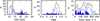 |
Fig. E.4. Basic physical properties of the full GES (black) and FS (blue) stellar samples. The distribution of the stars with C, N, Mg, or Si abundances from the FS is shown as a filled, blue histogram. |
As seen in Fig. E.5, a comparison of the parameters for the stars in common leads to the conclusion that our surface gravities and abundances with respect to hydrogen are systematically larger by ∼0.15–0.20 dex on average. The abundance offset could (partly) arise from the larger microturbulences often adopted by the FS. The strongest outlier by far in terms of Teff and log g (GES 10355467–5813486 or FS 3293-032) is one of the fastest rotators in both samples (V sin i ∼ 350 km s−1) and a possible Be transient (McSwain et al. 2009). No abundances are determined in either case. Our much cooler Teff and lower log g are clearly in better agreement with the ROBGrid results. As discussed by Hunter (2008), the Teff adopted by the FS for this star is calibrated on the spectral type that is ill-determined (in the range B0.5–B1.5 Vn).
 |
Fig. E.5. Comparison between our results and those from the FS. The differences are expressed as this study minus FS. Our silicon abundances are based on Si III. The microturbulence was adjusted by Hunter et al. (2009) to derive the same Si abundance for each star in the cluster (see Hunter et al. 2007; Trundle et al. 2007). Only the Δξ data for the stars with abundances from both this study and the FS are shown. |
Appendix F: Reference parameters for benchmarks
Figure F.1 shows a Kiel diagram for the stars used as benchmarks in this study.
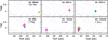 |
Fig. F.1. Reference position of the benchmark stars used in this study in the log g-Teff plane. Colour coding for literature values: Smith & Dworetsky (1993, yellow), Lefever et al. (2010, magenta), Simón-Díaz et al. (2006, green), Simón-Díaz (2010, dark green), Nieva & Simón-Díaz (2011, cyan), Nieva & Przybilla (2012, blue), Mokiem et al. (2005, sienna), Morel & Butler (2008, red), Hubrig et al. (2008, red), and Martins et al. (2012, orange). The average, adopted parameters are shown as a black cross. Evolutionary tracks at solar metallicity and with ωinit = 0.568 are overlaid (Ekström et al. 2012). The initial stellar mass (in solar units) is indicated. |
All Tables
Colour excesses and stellar parameters (pnrc, averaged over the stellar surface, and apparent).
Mean abundances for NGC 3293 compared to the solar photospheric values (Asplund et al. 2021) and previous non-LTE spectroscopic studies in the literature.
Results of the spectroscopic analysis based on iDR3 data for three representative exposures of GES 10354072–5812440.
All Figures
|
Fig. 1. Breakdown of the parallaxes for the stars with well-behaved astrometric solutions before (top panel) and after (bottom panel) applying the zero-point offsets of Lindegren et al. (2021a). A foreground star (GES 10344563–5813091) with a much larger parallax is off scale. The dashed lines show the mean values, while the dotted lines indicate the 3-σ thresholds. |
| In the text | |
|
Fig. 2. Astrometric and photometric properties of our sample. Red symbols highlight in all panels stars assumed not to be cluster members, while dark blue symbols indicate stars with possible issues with the Gaia EDR3 data. Left panels: proper motions. A typical error bar with a size multiplied by ten is shown. Top middle panel: parallax distribution. The dashed line shows our mean value. Bottom middle panel: coordinates (epoch J2000). Right panel: CMD. |
| In the text | |
|
Fig. 3. Time sampling. Breakdown of number of independent epochs, Nb (top panel), total time span of observations, ΔT (middle panel), and time interval between consecutive epochs, δT (bottom panel). |
| In the text | |
|
Fig. 4. Breakdown of the mean S/N of the epoch spectra. The S/N is computed by the GES and refers to the value averaged across the entire wavelength range. The histogram for U520 is multiplied by five for better visibility. |
| In the text | |
|
Fig. 5. Histograms of the normalised difference RV(HR03)–RV(HR04) (left panel) and RV(HR03)–RV(HR05) (right panel) for all the pairs. All the objects are included in the black histograms. The green histograms only include the contemporaneous pairs. The red continuous lines represent a Gaussian PDF of zero mean, μ, and with either unit variance (left panel) or σ = 1.414 (right panel). GES 10352851–5812496 is off scale in the right panel. |
| In the text | |
|
Fig. 6. Distribution of the mean RVs for the stars considered as constant. The red histogram is for stars assumed not to be cluster members, while the orange one is for the presumed members with the right parallax, but a discrepant proper motion (Sect. 3.3). The other stars are shown in black. The mean values found by Evans et al. (2005) and Soubiran et al. (2018) are shown as dashed and dotted lines, respectively. |
| In the text | |
|
Fig. 7. Variations of the dispersion in the Mg and He abundances (colour coded) as a function of Teff and V sin i. |
| In the text | |
|
Fig. 8. HR diagrams using apparent (top panel) and averaged over the stellar surface (bottom panel) stellar parameters. Isochrones for various ages and initial rotation rates are overlaid (Georgy et al. 2013). |
| In the text | |
|
Fig. 9. Rotational velocity distributions. (a) Histogram (grey) and smoothed distribution (blue) of (V sin i)app. The Vapp distribution is shown in red; (b) same as left panel, but for rotational velocities corrected for GD; (c) histogram (grey) and smoothed distribution (blue) of velocity ratios corrected for GD, (V sin i/Vc)pnrc. The distribution of GD-corrected velocity ratios, (V/Vc)pnrc, is shown in red. |
| In the text | |
|
Fig. 10. Stellar mass and inclination angle distributions. (a) pnrc masses; (b) inclination angles compared to the theoretical distribution for values at random. |
| In the text | |
|
Fig. 11. Distribution of stellar ages derived from ‘apparent’ (red) and corrected for GD (blue) fundamental parameters. |
| In the text | |
|
Fig. 12. Variations of the abundances as a function of the apparent stellar parameters. Non cluster-members (Sect. 3.3) were excluded. Stars with or without a binary flag are shown with open and filled symbols, respectively. Stars flagged or not as line-profile variables are plotted as squares and circles, respectively. For both variability types, a confidence level ‘A’ or ‘B’ is required. The benchmarks are shown with star symbols (for convenience, the position of those discussed in Sect. 7.3 is indicated in the panels showing the behaviour of the N and [N/C] abundances as a function of Teff). Crosses show illustrative error bars. The Si II and Si III data are plotted together in the same panels. The horizontal, dashed line indicates the solar abundance (Asplund et al. 2021), while the horizontal stripe shows the mean values (±1σ) for stars in NGC 3293 determined by Hunter et al. (2009). The values are provided in Table 6. The rightmost panels show the breakdown of our abundance data for the NGC 3293 sample. |
| In the text | |
|
Fig. 13. Distributions for each abundance ratio of the residuals with respect to the mean values (Table 6). Non cluster-members (Sect. 3.3) were excluded. A normal distribution with a standard deviation corresponding to the mean of our final random uncertainties is overplotted with a dashed line. The two stars with peculiar abundances are indicated in red. |
| In the text | |
|
Fig. 14. Model dependence between the current ω and mass for log(t) = 7.3 (Georgy et al. 2013). The behaviour is shown for rotation rates at birth, ωinit, ranging from 0.1 to 0.95. The observed ω and M values for the stars with and without [N/C] data are overplotted as filled circles and open squares, respectively. For clarity, only the former are shown with error bars. The star GES 10355661–5812407 is off scale because of a spuriously large mass. |
| In the text | |
|
Fig. 15. Comparison in a HR diagram between the [N/C] data (squares) and the predictions (circles) of solar-metallicity evolutionary models for various initial rotation rates and two cluster ages: log(t) = 7.2 (left panels) and 7.4 (right panels). The model predictions are taken from Georgy et al. (2013). The stars selected in each panel fulfil the condition |ω − ωinit| < 0.1. The observational error bars are smaller than the square symbols. The [N/C] abundance ratio is colour coded. The stars V380 Car – and to a lesser extent V405 Car – whose observations are at odds with the model predictions are indicated. |
| In the text | |
|
Fig. A.1. Comparison between our stellar parameters and those recommended by the GES. The differences are expressed as this study minus recommended. All the stars are shown irrespective of their membership status (Sect. 3.3). |
| In the text | |
|
Fig. B.1. Superposition of the GES UVES exposures of GES 10354072–5812440 for the spectral range encompassing the Si IIIλ4553 line profile. The exposure ID and MJD are indicated. |
| In the text | |
|
Fig. C.1. Example of spectral fits for the cool, slow rotator GES 10353450–5813461 with Teff = 11 760 K and V sin i = 42 km s−1 (top left panel), the cool, fast rotator GES 10353820–5811092 with Teff = 10 800 K and V sin i = 276 km s−1 (top right panel), the hot, slow rotator GES 10355660–5811314 with Teff = 22 701 K and V sin i = 27 km s−1 (bottom left panel), and the hot, fast rotator GES 10360349–5814401 with Teff = 20 322 K and V sin i = 257 km s−1 (bottom right panel). The observations are shown in black and the fits in red. Two stars do not have HR04 data available. |
| In the text | |
|
Fig. E.1. Comparison of results from repeated observations. Top panel of each sub-figure: differences between the results obtained using GES or FS data based on either GIRAFFE or UVES. Bottom panel of each sub-figure: differences between the results obtained using either UVES or GIRAFFE data. Two cases are considered: only GES data or observations taken from a different source (FS or GES). All the differences are expressed as GES minus FS and UVES minus GIRAFFE. The dotted curve is a normal distribution with a variance set to the nominal random uncertainty. |
| In the text | |
|
Fig. E.2. Comparison for a set of GES benchmarks between our mean results and those taken from the literature (Pancino et al. 2017; Blomme et al. 2022b). The differences are expressed as this study minus reference. The error bars along the vertical axis are the quadratic sum of our internal uncertainties and those in the reference values. The latter are assumed to be 500 K and 0.1 dex for Teff and log g, respectively. |
| In the text | |
|
Fig. E.3. Comparison with the results of other WG13 nodes. Left panels: differences between the stellar parameters expressed as this study minus other node. In each panel, fast rotators for which we estimate V sin i above 150 km s−1 are indicated by lighter colours. Only one colour is used for the ON node because only slow rotators below that threshold were analysed. Right panels: position of each sub-sample in a Kiel diagram based on our parameters. Theoretical evolutionary tracks at solar metallicity and with ωinit = 0.8 (see Sect. 6 for definition) are overlaid (Georgy et al. 2013). The initial stellar mass (in solar units) is indicated. |
| In the text | |
|
Fig. E.4. Basic physical properties of the full GES (black) and FS (blue) stellar samples. The distribution of the stars with C, N, Mg, or Si abundances from the FS is shown as a filled, blue histogram. |
| In the text | |
|
Fig. E.5. Comparison between our results and those from the FS. The differences are expressed as this study minus FS. Our silicon abundances are based on Si III. The microturbulence was adjusted by Hunter et al. (2009) to derive the same Si abundance for each star in the cluster (see Hunter et al. 2007; Trundle et al. 2007). Only the Δξ data for the stars with abundances from both this study and the FS are shown. |
| In the text | |
|
Fig. F.1. Reference position of the benchmark stars used in this study in the log g-Teff plane. Colour coding for literature values: Smith & Dworetsky (1993, yellow), Lefever et al. (2010, magenta), Simón-Díaz et al. (2006, green), Simón-Díaz (2010, dark green), Nieva & Simón-Díaz (2011, cyan), Nieva & Przybilla (2012, blue), Mokiem et al. (2005, sienna), Morel & Butler (2008, red), Hubrig et al. (2008, red), and Martins et al. (2012, orange). The average, adopted parameters are shown as a black cross. Evolutionary tracks at solar metallicity and with ωinit = 0.568 are overlaid (Ekström et al. 2012). The initial stellar mass (in solar units) is indicated. |
| In the text | |
Current usage metrics show cumulative count of Article Views (full-text article views including HTML views, PDF and ePub downloads, according to the available data) and Abstracts Views on Vision4Press platform.
Data correspond to usage on the plateform after 2015. The current usage metrics is available 48-96 hours after online publication and is updated daily on week days.
Initial download of the metrics may take a while.