| Issue |
A&A
Volume 690, October 2024
|
|
|---|---|---|
| Article Number | A151 | |
| Number of page(s) | 16 | |
| Section | Extragalactic astronomy | |
| DOI | https://doi.org/10.1051/0004-6361/202449187 | |
| Published online | 04 October 2024 | |
Application of the Eddington inversion method to constrain the dark matter halo of galaxies using only observed surface brightness profiles
1
Instituto de Astrofísica de Canarias, c/ Vía Láctea s/n, E-38205 La Laguna, Tenerife, Spain
2
Departamento de Astrofísica, Universidad de La Laguna, E-38203 La Laguna, Tenerife, Spain
3
CeBio y Departamento de Ciencias Básicas, Universidad Nacional del Noroeste de la Prov. de Buenos Aires, UNNOBA, CONICET, Roque Saenz Peña 456, Junin, Argentina
Received:
8
January
2024
Accepted:
22
July
2024
Context. The halos of low-mass galaxies may allow us to constrain the nature of dark matter (DM), but the kinematic measurements needed to diagnose the required properties are technically extremely challenging. However, the photometry of these systems is doable.
Aims. Using only stellar photometry, we wanted to constrain key properties of the DM halos in low-mass galaxies.
Methods. Unphysical pairs of DM gravitational potentials and starlight distributions can be identified if the pair requires a distribution function, f, that is negative somewhere in the phase space. We used the classical Eddington inversion method (EIM) to compute f for a battery of DM gravitational potentials and ∼100 observed low-mass galaxies with M⋆ between 106 and 108 M⊙. The battery includes Navarro, Frenk, and White (NFW) potentials (expected from cold DM) and potentials stemming from cored mass distributions (expected in many alternatives to cold DM). The method assumes spherical symmetry and an isotropic velocity distribution and requires fitting the observed profiles with analytic functions, for which we used polytropes (with zero inner slope, also known as core) and profiles with variable inner and outer slopes. The validity of all these assumptions is analyzed.
Results. In general, the polytropes fit the observed starlight profiles well. If they are the correct fits (which could be the case), then all galaxies are inconsistent with NFW-like potentials. Alternatively, when the inner slope is allowed to vary for fitting, between 40% and 70% of the galaxies are consistent with cores in the stellar mass distribution and thus inconsistent with NFW-like potentials.
Conclusions. Even though the stellar mass of the observed galaxies is still not low enough to constrain the nature of DM, this work shows the practical feasibility of using the EIM technique to infer DM properties only from photometry.
Key words: galaxies: dwarf / galaxies: fundamental parameters / galaxies: halos / galaxies: photometry / galaxies: structure / dark matter
Corresponding author; [email protected]
© The Authors 2024
 Open Access article, published by EDP Sciences, under the terms of the Creative Commons Attribution License (https://creativecommons.org/licenses/by/4.0), which permits unrestricted use, distribution, and reproduction in any medium, provided the original work is properly cited.
This article is published in open access under the Subscribe to Open model. Subscribe to A&A to support open access publication.
1. Introduction
The classical Eddington inversion method (EIM; Eddington 1916; An & Evans 2006; Binney & Tremaine 2008; Lacroix et al. 2018; Ciotti 2021) can be used to constrain the shape of the dark matter (DM) halo of a galaxy using only the observed stellar mass distribution. It provides the distribution function (DF) in the 6D phase space to be followed by a given mass density profile immersed in a given gravitational potential. The minimal requirement for any feasible DF is to be nonnegative everywhere in the phase space, and this seemingly simple constraint is enough to discard as unphysical many combinations of density and potential leading to a DF < 0. Recently, Sánchez Almeida et al. (2023) used the EIM in the regime of low-mass galaxies, where the contribution of the baryons to the overall potential can be neglected and the potential is set only by the DM. Among other results, they showed that cored stellar mass distributions (i.e., with a constant density when the distance to the center goes to zero) are inconsistent with the Navarro, Frenk, and White (NFW) potential expected in DM-dominated systems with collision-less cold DM (the so-called NFW profiles; Navarro et al. 1997). Strictly speaking, this result holds for spherically symmetric particle systems with an isotropic velocity distribution; however, extensions that relax these assumptions and yield similar constraints exist (a detailed account is given in Sect. 2.1).
The technique has great potential since, using only photometry, it may be able to constrain the shape of the DM halos in ultra-low-mass galaxies. In this mass regime, the baryon feedback is unable to turn cuspy DM halos into cored halos. Thus, if the DM halos of these galaxies happen to have a core, it will indicate a departure of the DM from being collision-less, reflecting the much sought-after presently unknown true nature of DM (whether it is fuzzy, self-interacting, warm, or other alternatives; e.g., Dodelson & Widrow 1994; Hu et al. 2000; Spergel & Steinhardt 2000; Bechtol et al. 2022; Carr et al. 2023). The stellar mass limit defining ultra-low-mass galaxies (i.e., the largest mass unable to modify the DM profile) is model dependent (e.g., Read et al. 2016). However, it roughly corresponds to a stellar mass of M⋆ < 106 M⊙ or a DM halo mass of Mh < 1010 M⊙ (e.g., Di Cintio et al. 2014b; Chan et al. 2015; Hayashi et al. 2020; Jackson et al. 2021; Expósito-Márquez et al. 2023). Traditionally, halo shapes are deduced from kinematical measurements, which require high spectral resolution spectroscopy and which, keeping in mind the need for large statistics to derive firm conclusions on the nature of DM, are virtually impossible in this ultra-low-mass regime. However, the broadband photometry needed to infer their stellar mass profiles is becoming increasingly feasible (e.g., Trujillo et al. 2021) and will be routinely simple in the near future with instruments such as the Rubin Observatory (Ivezić et al. 2019). Here is where the EIM comes into play, constraining the properties of the halo mass distribution from the stellar light alone.
The present work represents the first application of the EIM-based technique devised by Sánchez Almeida et al. (2023) to real galaxies. We present diagnostic diagrams and discuss the kinds of constraints to be expected in practice. The target galaxies were collected by Carlsten et al. (2021, 2022) to represent dwarf satellites of Milky Way-like galaxies. This sample is not ideal for ascertaining the nature of DM since (1) their masses exceed the 106 M⊙ limit and (2) the fact that they are satellites complicates the interpretation of the DM halo shape in terms of the DM nature alone. The evolution of satellites may be influenced by the central galaxy through tidal forces and gas pressure gradients (e.g., Lan et al. 2016; Sánchez Almeida et al. 2017). However, this galaxy set is a good testbed since it comprises a large number of objects (≳100) with density profiles comparable, in terms of their lack of symmetry and noise, with those to be expected soon for the appropriate galaxies.
The paper is structured as follows: Sect. 2 summarizes the technique to be employed, with Sect. 2.1 giving an overview of the EIM, including an extension that goes beyond the spherical symmetry assumption (Appendix B). The actual algorithm is described in Sect. 2.2, and then tested in Appendix C. The data are presented in Sect. 3, with the new diagnostic diagrams detailed in Sect. 4. These diagrams depend on the functions used for fitting the observed profiles. For this task, we first use projected polytropes in Sect. 5.1. Polytropes have cores, an assumption relaxed in Sect. 5.2 (free inner slope fits) and Sect. 5.3 (free inner and outer slope fits). Our conclusions are analyzed in Sect. 6, including the impact of the assumptions made when we applied the EIM, such as spherical symmetry and isotropic velocity distributions.
2. The Eddington inversion method (EIM)
For the sake of comprehensiveness, and to set the scene, Sect. 2.1 gives a brief account of the EIM and the implications for low-mass galaxies found by Sánchez Almeida et al. (2023). Then the practical application of the method carried out in the present paper is explained in Sect. 2.2.
2.1. Contextual briefing of the EIM
For spherically symmetric systems of particles with isotropic velocity distribution, the phase-space DF f(ϵ) depends only on the particle energy ϵ. The space density ρ(r) is an integral over all velocities v at a fixed distance r. If Ψ(r) = Φ0 − Φ(r) is the relative potential energy, then the relative energy (per unit mass) is  , so that the density becomes (e.g., Binney & Tremaine 2008, Sect. 4.3)

with Φ(r) the gravitational potential and Φ0 its value at the edge of the system. For realistic systems, the relative potential Ψ is a monotonically decreasing function of the distance from the center r. Consequently, ρ can be regarded as a function of Ψ. Differentiating ρ with respect to Ψ yields
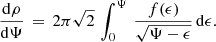
Inverting this Abel integral and after some mathematical manipulations, one finds the equation for f(ϵ) in terms of the spatial density,

which provides the renowned EIM equation. It gives the DF f(ϵ) consistent with ρ and Φ.
However, given an arbitrary pair of ρ and Φ (or ρ and Ψ), it is not guaranteed that the DF yielded by Eq. (3) is positive everywhere in the phase space. If f < 0 somewhere it means that this particular combination of ρ and Φ cannot exist in practice. Sánchez Almeida et al. (2023) analyze a sizable set of pairs ρ − Φ showing a number of inconsistencies that may be important for real galaxies. The simplest one, yet very powerful, directly follows from Eq. (2). If dρ/dΨ = 0 then the integral in the right hand side of Eq. (2) has to be zero so that f(ϵ) < 0 somewhere within the interval 0 ≤ ϵ ≤ Ψ. This is precisely what happens with any cored density profile immersed in a NFW potential. Since the only variable is r,

A cored mass density is defined to have

which is inconsistent with a NFW background potential, which has

The above conclusion holds for spherically symmetric systems with isotropic velocity distribution; however, this restriction can be relaxed to accommodate more general systems. Surpassing the simplest assumption requires treating particular cases individually, each one with its own peculiarities; therefore, only a handful of them have been analyzed so far, probably representing the tip of the iceberg. In order to discuss these individual cases, it is necessary to define the velocity field anisotropy parameter, β,

where σvr and σvt are the radial and tangential velocity dispersion, respectively. The isotropic systems leading to the EIM Eq. (3) have σvt2 = 2σvr2 and so β = 0. Systems with radially biased orbits have β > 0 whereas systems with tangentially biased orbits have β < 0. Systems with circular orbits, having σvr = 0 and therefore β = −∞, are a limiting case of the latter. The case where

is called the Osipkov-Merritt model and introduces a new characteristic length scale rb. It is tractable analytically and approximately describes the global trend expected in low-mass galaxies, with β ∼ 0 in the center and then increasing outward (β > 0).
The constraints on the potential imposed by the stellar mass distribution are best described in terms of the inner logarithmic slope of the stellar density profile, c,

and the inner slope of the total mass density profile, ρp, which defines the gravitational potential,

The univocal association between Ψ and ρp is granted through the Poisson’s equation, which, for spherically symmetric systems, yields (e.g., An & Zhao 2013)
![$$ \begin{aligned} \Psi =4\pi G\,\left[\frac{1}{r}\,\int _{0}^r\,t^2\,\rho _p(t)\,\mathrm{d}t+\int _r^{\infty }\,t\,\rho _p(t)\,\mathrm{d}t\right]. \end{aligned} $$](/articles/aa/full_html/2024/10/aa49187-24/aa49187-24-eq12.gif)
In terms of c and cp, a cored stellar density profile has c = 0 whereas a NFW potential has cp = 1. From now on, the term “soft-core” is used to denote those profiles where the inner slope is not exactly zero but close to it (c or cp ≳ 0). Equipped with these definitions, the main known constraints imposed by the EIM are (Sánchez Almeida et al. 2023):
-
Stellar cores (c = 0) and NFW potentials are incompatible, provided the velocity distribution is isotropic (β = 0). This was already proven above.
-
Stellar cores are also incompatible with potentials stemming from a total density with a quasi-core (cp > 0) for β = 0.
-
As expected for physical consistency, stellar cores (c = 0) and potentials resulting from cored density profiles (cp = 0) are consistent in isotropic (β = 0) and radially biased systems (β > 0).
-
Stellar cores and NFW potentials are also incompatible in systems with anisotropic velocities following the Osipkov-Merritt model.
-
Stellar cores and NFW potentials are incompatible in systems with radially biased orbits (constant β > 0). Actually, a stellar core is incompatible with any potential without a core in systems with constant radially biased orbits (β > 0).
-
Circular orbits (β = −∞) can accommodate any combination of baryon density and potential, including a cored stellar density in a NFW potential. However, this configuration is very artificial from a physical standpoint.
-
A convex linear combination of two DFs that are both consistent with a given potential constitutes a new DF that is also consistent with the same potential. Thus, one may think that adding a positive DF for circular orbits may compensate a negative DF for isotropic orbits to yield a positive physically sensible DF. However, this is not the case. Independently of the relative weight, the superposition of an unphysical DF for isotropic velocities (β = 0) with a physically realizable DF for circular orbits (β = −∞) always yields unphysical DFs.
-
Soft-cores are inconsistent with NFW potentials when c ≲ 0.1 while they are consistent when c ≳ 0.1.
-
The inner slope of a soft stellar core and the radial anisotropy are related so that c > 2β for the system to be consistent. In other words, systems with radially biased orbits are inconsistent with soft stellar cores.
-
Positive inner slope in the stellar distribution (c < 0), where the density grows outward, is discarded in every way for isotropic velocity.
-
For stellar densities and potentials with the same shape (whether cored or not), the stellar density distribution cannot be broader than twice the width of the density characterizing the potential. This result refers to isotropic velocities and may be used in real galaxies to set a lower limit to the size of the DM halo from the size of the observed starlight.
-
The above results do not depend on a global factor scaling the stellar density profile; therefore, they do not depend on the (unknown) ratio between the stellar mass and the total mass of the system. Moreover, it implies that light profiles or star number counts could replace mass density in the EIM.
To the above list of known constraints, here we add another one relaxing the l symmetry assumption. In Appendix B we prove that the incompatibility between NFW potentials and stellar cores also holds for axisymmetric systems of arbitrary axial ratio. It is particularly relevant because this fact shows how the incompatibility goes beyond the spherical symmetry assumption, being more fundamental than, and not attached to, this particular hypothesis.
2.2. Procedure followed in this study
As summarized in Sect. 2.1, the EIM gives the DF f needed for the stellar density profile ρ to reside in a gravitational potential Φ. If two arbitrary ρ and Φ yield f < 0 somewhere in the phase space, this particular combination is physically inconsistent and can be discarded. Here we apply the technique to constrain the properties of the halos in a number of observed galaxies. The procedure works as follows:
-
Measure Σo in a real galaxy, that is, the projection along the line of sight (LOS) of the density ρo.
-
Fit Σo with a synthetic Σ to estimate ρo (i.e., the ρ whose Σ best fits Σo). For spherically symmetric systems, the relation between ρ and Σ is univocal (e.g., Binney & Tremaine 2008),
with R the projected distance to center of the system.
-
Using the EIM (Eq. (3)), compute the foi corresponding to the ρ best fitting ρo and a battery of Φi, with i = 1, 2, …
-
Discards as unphysical, all the Φi that yield foi < 0 somewhere in the phase space.

The above algorithm can be applied to individual galaxies as well as to sets of them (o = 1, 2, …). For example, one can compute the fraction of times that a fixed Φi is unphysical considering all the galaxies in a particular set. This is the approach followed in our work, which requires the computation of foi for all galaxies in the set (∀o) and for all potentials (∀i). Then we use the fraction of times that it is consistent (i.e., the fraction of times where foi ≥ 0 everywhere) as a diagnostic for the reliability of the potential Φi. Practical examples of the procedure are given in Sect. 4.
This scheme has been tested for consistency using the set of globular clusters (GCs) collected by Miocchi et al. (2013). In general, GCs are known to have little or no DM (e.g., Sollima et al. 2012; Ibata et al. 2013); therefore, GCs can be regarded as self-gravitating systems so that the gravitational potential is set directly by the observed stellar distribution. Moreover, the stellar surface density of GCs usually show cores. Thus, GCs are excellent testbeds for our EIM-based approach since it provides constraints on the properties of the potential that can be directly compared with the true values obtained from the surface density profile. The tests are detailed in Appendix C, and they lead to the conclusion that our scheme gives consistent results with the gravitational potential of the GCs inferred from their stellar distribution.
3. Observed profiles and fits
This section describes the practical realization of steps number 1 and 2 in the procedure described in Sect. 2.2.
The observed surface density mass distributions analyzed in the paper come from Carlsten et al. (2021, 2022). They provide the surface brightness profile in the g band (μg) for a set of dwarf satellites of Milky Way-like galaxies. They use photometry from various existing surveys including the DESI Legacy Imaging Surveys (Dey et al. 2019) and the Beijing–Arizona Sky Survey (Zou et al. 2017, 2018; see Carlsten et al. 2021 for details). The galaxies are low-mass dwarfs with stellar masses between 106 and 108 M⊙ as inferred from integrated photometry (Into & Portinari 2013). The profiles are shown in Fig. 1, with the faintest signals in the outskirts reaching down to 30 mag arcsec−2. Even though the sky subtraction was carefully carried out using ad hoc custom-made procedures (Carlsten et al. 2019), one cannot discard over or under corrections in the faint end of the profiles (μg ≳ 29 mag arcsec−2).
 |
Fig. 1. Surface brightness profiles in the g band for the early-type galaxies in Carlsten et al. (2021, 2022). The left panel shows stellar masses between 106 and 107 M⊙, whereas the right panel corresponds to masses between 107 and 108 M⊙. Note how the profiles tend to present a central plateau or core. This color code is maintained in Figs. 6, 10, and 14. |
In principle, the EIM requires knowing the stellar mass density to be applied, but we use μg directly because the shape of the DF is independent of a scaling factor in Σo (Sect. 2.2) and

with ℵ the mass-to-light ratio. Obviously, for Σo to scale as the surface brightness F, ℵ has to be constant along the profile, which is a fair assumption for early-type galaxies, and the reason why we only used the early-type galaxies in Carlsten et al. (2021) for our analysis1. Carlsten et al. (2021) classified early and late-type galaxies by eyeball inspection of their morphology so that smooth featureless objects are early types while objects with star-forming regions, blue clumps, or dust lanes are late types. The original set contains 111 early-type galaxies, but it was additionally purged to leave 93 as described in Sect. 4.
The volume density profiles required to compute the phase-space DF through the EIM (Eq. (3)) are found by fitting various surface density profiles to the observed −μg/2.5. The fits are carried out using a least-squares minimization routine based on the Levenberg–Marquardt algorithm, reproducing the procedure employed in Sánchez Almeida et al. (2021). We start off from a family of volume density profiles ρξ(r), with ξ representing the free parameters that characterize the profile. Even when ρξ(r) is analytical, its 2D projection is not; therefore, Eq. (12) has to be evaluated numerically to carry out the fits. To speed up the procedure, the surface densities required for fitting result from interpolating on a precomputed grid Σξ(R), related to ρξ(r) through Eq. (12). We employ a linear interpolation in as many dimensions as needed to account for the number of free parameters defining ρξ(r). The fits do not include the effect of the point-spread-function (PSF) on the shape of the synthetic profiles since the observed profiles are well resolved, even at the innermost radius (100 pc, Fig. 1). At the average distance of the observed galaxies (∼7 Mpc), 100 pc corresponds to 3″, which is significantly larger than the typical width of the PSF (≲1″; Carlsten et al. 2021).
Figure 2 shows examples of this kind of fit to profiles in Fig. 1, where the density is fitted using polytropes. In this case the profiles depend on three parameters: a global density scaling, a spatial scaling rs, and the polytropic index m (see Sánchez Almeida et al. 2021). Polytropes are relevant in this context because they represent self-gravitating systems of maximum Tsallis entropy and so they describe the thermodynamical equilibrium of systems experiencing long-range forces (Plastino & Plastino 1993; Sánchez Almeida 2022b). Polytropes are know to describe the distribution of DM observed in dwarf galaxies (Sánchez Almeida et al. 2020), the starlight observed in galaxies of various masses (Sánchez Almeida et al. 2021), as well as the DM distribution in numerical simulations of self-gravitating systems reaching thermodynamical equilibrium (Sánchez Almeida & Trujillo 2021).
Figure 2 shows both good (top three rows) and bad (bottom row) fits to some of the observed profiles. The quality control parameter, called ‘Relative RMS” in Fig. 2 and throughout the text, is defined as

 |
Fig. 2. Examples of projected polytrope fits to some of the profiles in Fig. 1. The first three rows contain good fits. The bottom row shows examples of bad fits, usually profiles with bumps resulting from deviations from axial symmetry of the original galaxies. The blue dots represent the observed points, whereas the orange line shows the fit, which is solid or dashed depending on whether it is within or outside the range of fitted radii. The secondary subpanel in each panel shows the residuals of the fit. The insets provide information on the galaxy and the fit. |
with RMS the root mean square of the residuals of the fit and log F the logarithm of the observed flux (Eq. (13)). It represents the error in the fit relative to the amplitude of the observed signal. It is a good proxy for the quality of the fits so that a Relative RMS ≃ 0.02 separates the good fits (< 0.02) form the fair fits (> 0.02) as judged rather arbitrarily from the eye-ball inspection of the individual fits (see Fig. 3).
 |
Fig. 3. Residuals of the fits to projected polytropes of the profiles shown in Fig. 1. The color code refers to the maximum Relative RMS defining each set of profiles. What we define as “good” fits are shown in blue and orange. |
All polytropes have cores in the sense given in Eq. (5); therefore, to broaden the range of possibilities, we also tried other more flexible density profiles, namely, the ρabc profiles defined as

where x = r/rs, and ρs and rs are scaling constant in density and radius, respectively. These profiles are commonly used to model the density of baryons or DM (e.g., Hernquist 1990; Merritt et al. 2006; Di Cintio et al. 2014a) and have the advantage of encompassing the iconic NFW profile (a = 1, b = 3, and c = 1) and the m = 5 polytrope (also known as Schuster-Plummer profile, with a = 2, b = 5, and c = 0). Moreover, for a = 2, b = m, and c = 0,
![$$ \begin{aligned} \rho _{2m0} = \frac{\rho _s}{\left[1+(r/r_s)^2\right]^{m/2}}, \end{aligned} $$](/articles/aa/full_html/2024/10/aa49187-24/aa49187-24-eq17.gif)
it approximately accounts for the inner region of a polytrope of arbitrary index m (e.g., Sánchez Almeida 2022b). The ρabc profile is more flexible than the polytropes because the inner and outer slopes can be fitted independently: the parameter b encodes the outer logarithmic slope of the profile,

whereas c encodes the inner logarithmic slope (as in Eq. (9)). Examples of these alternative fits will be given later on in connection with the results (Sect. 5).
4. Diagnostic diagrams
This section describes the practical realization of steps 3 and 4 in the procedure sketched out in Sect. 2.2.
To constrain the properties of the gravitational potential, we computed for each observed profile the DFs in the phase-space corresponding to a battery of potentials. To make the interpretation intuitive, the potentials are described in terms the mass density profile that creates the potential ρp(r) (Eq. (11)). In general the relation between ρp and Ψ is not analytical and has to be computed numerically. For ρp we used a particular type of ρabc function (Eq. (15)),

that scans seamlessly from a Schuster-Plummer profile to a NFW profile when cp goes from 0–1. Thus, the potentials in the battery are defined in terms of the two free parameters that define ρp, cp and rsp. (The scaling factor ρsp is irrelevant for the EIM, as pointed out in Sect. 2.1.) The key question of the analysis is knowing whether the DF resulting from the observed profile and each potential is or not negative. The answer to the question can be summarized in the kind of diagnostic diagram shown in Fig. 4. Red dots correspond to f < 0 and so mark unphysical potentials whereas blue dots corresponds to f ≥ 0 and so trace gravitational potentials consistent with the density profile.
 |
Fig. 4. Constraints on the underlying potential inferred from the polytropic fit of a representative galaxy. The corresponding fit is shown in Fig. 2 (first column, second row). Each potential is characterized by two parameters, as shown in Eq. (18): the inner slope, cp, and the global spatial scale, rsp. Red dots correspond to f < 0 and so mark unphysical potentials, whereas blue dots correspond to f ≥ 0 and so trace potentials consistent with the density profile. The parameter rs gives the spatial scale of the stellar light distribution. The horizontal lines define NFW potentials (cp = 1; solid gray line) and cored potentials (cp = 0; dashed gray line). |
Figure 4 shows a typical example corresponding to galaxy #15, with good polytropic fit in Fig. 2. Here an throughout the paper f is computed using the methods and tools developed by Sánchez Almeida et al. (2023). These tools only work for ρabc profiles, therefore, for this calculation polytropes were approximated using Eq. (16). We note that all cp > 0 are discarded in Fig. 4. All potentials have to derive from a cored density profile to be consistent with the fitted polytropes. This comes with no surprise since all polytropes have a core (e.g., Sánchez Almeida et al. 2020) and we proved that a core in stars requires a core in the potential for spherically symmetric systems and isotropic velocity distributions (see details in Sect. 2.1). In addition, some of the models with rs ≥ rsp are also incompatible. We also knew from Sánchez Almeida et al. (2023) of the inconsistency of potentials with characteristic radii (rsp) significantly smaller than the stellar core radii (rs). Perhaps more surprising is the fact that no incompatibility is found for some potentials with cp < 0, where the total density goes to zero when r → 0. These potentials are included in the battery for comprehensiveness although they are expected to be Rayleigh–Taylor unstable (e.g., Sánchez Almeida 2022a) and so of difficult practical realization. Once again, Sánchez Almeida et al. (2023) showed that in this case (c = 0, a = 2, and cp < 0) the derivative dρ/dΨ > 0 when r → 0 and so there is no need for f to be negative (see their Appendix E).
From the 111 galaxies in Fig. 1, we discarded those with bad fits (like those of the bottom row in Fig. 2) and were left with 93 good and fair fits. For every one of these profiles, we have a diagnostic diagram like the example shown in Fig. 4. We constructed a second kind of diagnostic diagram to show the constraints on the underlaying potential imposed for the whole set of observed profiles. For every potential, characterized by cp and rs/rsp, we counted the frequency of f ≥ 0 considering all the observed galaxies. The result is shown in Fig. 5. As we knew, the whole region of cp > 0 is discarded by all (100%) of the fits. The region with cp ≤ 0 is permitted provided rsp ≳ rs/2. The results do not change much when only the good fits are used (Relative RMS < 0.02) or when only the low-mass galaxies are considered (M⋆ < 107 M⊙).
 |
Fig. 5. Constraints on the underlying potential imposed by the set of polytropic fits like to those shown in Fig. 2. Every potential is characterized by cp and rsp, and the color code shows the frequency of having f ≥ 0 considering all good and fair fits (93 galaxies). The whole region of cp > 0 is discarded, whereas cp ≤ 0 is permitted provided rsp ≳ rs/2. The diagram does not change much when only good fits are considered (Relative RMS < 0.02) or when only low-mass galaxies are selected (M⋆ ≤ 107 M⊙). The parameter rs gives the spatial scale of the stellar light distribution. Horizontal lines defining NFW potentials (cp = 1; solid gray line) and cored potentials (cp = 0; dashed gray line) are included. |
Formal error bars can be assigned to this kind of diagnostic diagram as follows. It is based on counting the number of galaxies that, for the same potential, do or do not have a particular property (i.e., whether or not f ≥ 0 everywhere). Thus, the actual number of counts should follow a binomial distribution. Using this idea, we work out in Appendix A the error bars to be expected. They are largest when the percentage is 50%, and tend to zero at 0% and 100%. The actual error depends on the number of galaxies employed in the diagram. For ∼50 galaxies (typical number of good galaxies or low-mass galaxies in our sample), it is smaller than 6% (Fig. A.1).
5. Results
Armed with the fits described in Sect. 3 and the diagnostic diagrams of Sect. 4, here we describe the constraints on the potentials set by the observed surface brightness profiles. The degrees of freedom in the fits increase from polytropes (Sect. 5.1) to variable inner slope (Sect. 5.2) to allow both the inner and outer slopes to vary simultaneously (Sect. 5.3).
5.1. Polytropic fits with zero inner slope
Examples of polytropic fits are shown in Fig. 2. The quality of these fits was quantified using the Relative RMS (Eq. (14)), and overall, the quality is satisfactory (see the residuals in Fig. 3). As we mentioned in Sect. 4, from the 111 original profiles in Fig. 1, 18 are discarded because the profile is not smooth and the fits are bad (like those of the bottom row of Fig. 2). From the remaining 93, 41 are good (44%, with Relative RMS < 0.02) and the rest fair (64%).
The results of the fits are summarized in Figs. 6 and 7. The top panel of Fig. 6 shows the dependence of the inferred polytropic index m as a function the quality of the fits parameterized by the Relative RMS. There seems to be a trend for the best quality polytropic fits to have m ∼ 5, a behavior also found in other galaxy samples (Sánchez Almeida et al. 2021). This trend does not depend on the stellar mass, divided into low- (≤107 M⊙) and high-mass (> 107 M⊙) bins for the plot. The middle panel of Fig. 6 contains the size of the core versus the goodness of the fit. No trend is found. The bottom panel of Fig. 6 shows the stellar mass versus the goodness of the fit, and there is a hint of trend so that fits are slightly better for the more massive galaxies. This effect may be an observational bias since more massive objects tend to be brighter and thus present better observations that leave smaller residuals. The top panel of Fig. 7 shows the polytropic index as a function the stellar mass of the galaxy. Overall, there is no clear trend of m with log M⋆, which may be due to the fact that the lowest-mass galaxies happen to have the worst fits where m is more uncertain. However, the good fits seem to indicate a trend for m to grow with increasing M⋆ (the blue symbols in Fig. 7, top panel). The middle panel of Fig. 7 displays the variation of the core radius with stellar mass. More massive galaxies tend to have larger cores. This trend does not depend on the quality of the fits, represented with two colors depending on whether the Relative RMS is smaller or larger than 0.02. The bottom panel of Fig. 7 shows the variation of the absolute RMS with stellar mass. We note that the good fits have an absolute RMS better than 0.03 dex, equivalent to 7% in flux.
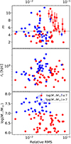 |
Fig. 6. Quantitative summary with the results of the polytropic fit to the profiles shown in Fig. 1. Low (≤107 M⊙) and high (> 107 M⊙) stellar mass galaxies are represented with a different color, as indicated in the bottom panel. Top panel: Dependence of the inferred polytropic index, m, on the quality of the fits, as parameterized by the Relative RMS. There seems to be a trend for the best quality fits to have m ∼ 5 (marked with the horizontal solid gray line). Middle panel: Scatter plot with the size of the core versus the goodness of the fit. Bottom panel: Scatter plot with the stellar mass versus the goodness of the fit. More massive galaxies lead to slightly better fits. |
 |
Fig. 7. Quantitative summary with the results of the polytropic fit to the profiles shown in Fig. 1. Medium- (Relative RMS > 0.02) and high-quality (≤0.02) fits are represented with different colors, as indicated in the bottom panel. Top panel: Scatter plot of the polytropic index, m, as a function of the stellar mass of the galaxy. Middle panel: Variation of the core radius with stellar mass. More massive galaxies tend to have larger cores. Bottom panel: Scatter plot with the variation of the absolute RMS with stellar mass. Good fits (blue dots) have absolute RMS ≲0.03 dex. |
With the polytropic fits described above, we constructed the diagnostic diagrams shown in Figs. 4 and 5. They were discussed as examples to present the diagnostic diagrams in Sect. 4, and there is little else to add except to emphasize that all kinds of cuspy potentials are discarded (cp > 0) and the characteristic radius of the potential cannot be significantly smaller than the radius of the stellar distribution (rsp ≳ rs/2). The first result was to be expected since given the hypotheses made in our application of the EIM, a core in stars necessarily needs of a core in the potential, and all polytropes are cored profiles independently of their index.
 |
Fig. 8. Fits similar to those shown in Fig. 2 but allowing the inner slope of the stellar mass profile to vary (dashed green lines) and the inner and outer slopes to vary independently (orange lines). The density used for the fitting was assumed to be ρabc in Eq. (15) with different bonds between a, b, and c for the green and orange lines. See the main text and the caption of Fig. 2 for further details. |
5.2. Variable inner slope fits
Going a step further, we no longer force a core in the stellar density profile, and the fits allows for a inner slope different from zero. The shape of the stellar density profiles is taken from Eq. (18), which scans from cored to NFW profiles when the inner slope c goes from 0–1. Examples of these fits are shown as green dashed lines in Fig. 8, which contains exactly the same galaxies as Fig. 2. In general, the fits using projected polytropes seem to do a slightly better job than these other fits, even though the number of free parameters is the same in both cases: m has been replaced with c. This may be due to the fact that polytropes, rather than ρabc profiles, are to be expected when self-gravitating systems reach thermodynamic equilibrium (Plastino & Plastino 1993). Figure 9 shows a scatter plot between the Relative RMS obtained with the two types of fit. Even if the differences are not overwhelming, the polytropic fits tend to be better than for these other fits. The fraction of good fits (Relative RMS < 0.02) is larger for polytropes than for the variable inner slope fits (44% versus 32%). Considering only good and fair fits, polytropic fits have lower Relative RMS in 59% of the cases. Finally, the number of times where the polytropic fits are significantly better than the alternative (defined as ratio of Relative RMS > 1.5) is much larger than the opposite (19 galaxies versus 3 galaxies).
 |
Fig. 9. Scatter plot of the Relative RMS resulting from variable inner slope fits and from polytropic fits. Different colors designate different qualities of the polytropic fits (see the inset). The points corresponding to low-mass galaxies are encircled in red. The absolute number of good polytropic fits is larger, as is the relative fraction of good over bad fits. |
The properties of the variable inner slope fits are summarized in Figs. 10 and 11. The top panel of Fig. 10 shows the dependence of the inner slope c as a function the Relative RMS. We note that often the best fitting c is negative. Most of these negative slopes may be produced by systematic errors in the fit, a conjecture supported by two facts: (1) the number of galaxies with c < 0 increases with increasing Relative RMS (Fig. 10, top panel) and (2) polytropic fits, where c = 0 is imposed, often provide better fits, as discussed in the previous paragraph. The middle panel of Fig. 10 contains the size of the core versus the goodness of the fit. No obvious trend is found. The bottom panel of Fig. 10 shows the stellar mass versus the goodness of the fit indicating a hint of trend where more massive galaxies show better fits. The top panel of Fig. 11 shows a scatter plot of the inner slope c as a function the stellar mass. There is no clear trend. The middle panel of Fig. 11 displays the variation of the core radius with stellar mass. More massive galaxies tend to have larger cores, as it happened with polytropic fits (Fig. 7, middle panel). The bottom panel of Fig. 11 shows the variation of the absolute RMS with stellar mass.
 |
Fig. 10. Quantitative summary with the results of the variable inner slope fit. Except for the inner slope c, the rest is similar to Fig. 6 describing polytropic fits. Note how c is often negative, a trend that becomes more pronounced as the quality of the fits worsens. |
 |
Fig. 11. Quantitative summary with the results of the variable inner slope fit. Except for the inner slope c replacing the polytropic index, the figure is similar to Fig. 7 describing the polytropic fits. |
The diagnostic diagrams to constrain the properties of the gravitational potential consistent with these fits are shown in Fig. 12. Contrary to what happens with the polytropic fits, where most of the potentials are either allowed or forbidden (Fig. 5), most of the potentials are sometimes allowed and sometimes forbidden. The results for all galaxies are shown in the top panel of Fig. 12. Around 50% of the potentials are not allowed, with a formal error in this estimate on the order of 5–10% (Appendix A). This happens irrespectively of the inner slope of the potential cp, with the fraction increasing with increasing rs/rsp. As discussed above (Fig. 10, top panel), a significant part of the fitted profiles have c ≤ 0, and these profiles are inconsistent with any potential. The middle panel of Fig. 12 includes only good fits (Relative RMS < 0.02). The fraction of unphysical potentials is significantly reduced as expected following the reduction of objects with c < 0 (Fig. 10, top panel). The bottom panel of Fig. 12 shows only low-mass galaxies (M⋆< 107 M⊙). This other time the fraction of unphysical potentials increases due to the increase in the percentage of fits with c < 0 among low-mass objects. Thus, we suspect that the diagnostic plots are significantly biased by the large uncertainty in c, which allows for many potentials to either be consistent (c significantly larger than 0) or inconsistent (c < 0). The shape chosen for fitting does not constrain the central slope of the observed galaxy well enough. Or equivalently, the errors (stochastic and systematic) are still not small enough to reach a solid conclusion. We note that the scenario does not change significantly even when the Relative RMS is chosen as small as < 0.01 (Fig. 3). In the next section, we try another type of fit to check whether it improves the situation. The fitting functions used here tie the inner and outer slopes of the density profile, and this artificial bound may be causing significant systematic errors.
 |
Fig. 12. Constraints on the underlying gravitational potential imposed by the variable inner slope fits. Top panel: Diagnostic diagram, equivalent to Fig. 5 for the polytropic fits, which includes all galaxies together. Note that around half of the galaxies have unphysical f < 0 irrespectively of the inner slope of the potential (cp), a percentage that increases as rs/rsp increases. This is mostly due to the inner slope, c, being negative for a number of galaxies. Middle panel: Same as the top panel but including only good fits (Relative RMS < 0.02). Note how the fraction of unphysical potentials with f < 0 has been significantly reduced (the tone becomes bluish rather than greenish). Bottom panel: Same as the top panel but including only low-mass galaxies (M⋆< 107 M⊙). As expected, the fraction of potentials with f < 0 increases (the tone becomes reddish) due to the increase in fits with c< 0. The color bar shows the percentage of galaxies with f ≥ 0. |
5.3. Variable inner and outer slopes
Even though the variable inner slope profiles have the same number of free parameters as the polytropic fits, they tend to provide slightly worst fits (Fig. 9). The problem could be due to the fact that the inner slope in these fits, c, also sets the outer slope, b = 5 − 2c (cf. Eqs. (15) and (18)). This tie minimizes the number of free parameters in the fit, but there is no clear physical reason to expect it. To overcome the potential problem created by the artificial link between b and c, we carried out additional fits where both the inner and outer slopes in Eq. (15) are free parameters. The third parameter of the abc profiles, a, which determines the transition between the inner and outer parts, are set to 2, which is the value corresponding to the polytropes2 (Eq. (16)). Examples of fits with free inner and outer slopes are shown as orange lines in Fig. 8. The figure also includes the fits with variable inner slope only (dashed green lines). Even though the Relative RMS is lower when both c and b are free parameters (top panel, Fig. 13), the fitted profiles look very similar, and also similar to the observed profiles (Fig. 8). Figure 14 shows how c and b depend on the Relative RMS of the fit.
The constraints on the gravitational potential imposed by these fits are similar to those when only the inner slope is free (Fig. 12). There is no major qualitative difference. A significant part of the fits still render c ≤ 0 and therefore unphysical f < 0 DFs. The galaxies can be divided into those with c ≳ 0.1, which are consistent with a NFW potential (cp = 1), and those with c ≲ 0.1, which are inconsistent (see Sect. 2.1). However, part of the scatter in c is probably artificial as deduced from the fact that the scatter increases with increasing Relative RMS (Fig. 14, top panel). The uncertainties in the fits are partly due to errors in the photometry but, most likely, the are systematic arising from deviations from the assumptions implicit in the fits, including spherical symmetry, ρabc profile, and a = 2. We tried to estimate the impact of these systematic errors on the inner slope c under the working hypothesis that all negative slopes c < 0 are due to noise. We selected all the profiles with good fits (Relative RMS < 0.02) and c < 0. If these values are random excursions produced by noise of profiles with c ≃ 0, then the standard deviation of the noise would be σc ≃ 0.3. (The same exercise with the fits in Sect. 5.2, where only the inner slope was fitted, renders σc ≥ 0.25.) Thus, we find that 38% of the good fits have |c|≤σc and therefore are consistent with c = 0 within errors. (The same exercise with the inner slope free fits renders 60%.) In other words, around 40% of the fits are consistent with cores in the stellar mass distribution (i.e., with c = 0) and so likely inconsistent with NFW-like potentials. This figure is also similar to the limit steaming from the diagnostic plot (e.g., Fig. 12, middle panel).
The Relative RMS of the free inner and outer slope fits is in general smaller than for polytropes (Fig. 13, bottom panel). However, the comparison of the two types of fits is not direct since two-slopes fits have one more degree of freedom than polytropes, and since the two shapes are different, an increase in the number of free parameters my artificially reduce the RMS because of overfitting. This being said, we find that the number of profiles with Relative RMS < 0.02 is very similar in both cases (41 for polytropic fits versus 39 for ρ2bc) so is the number of profiles with significantly better fit of one Relative to the other (10 versus 12). The similitude between the numbers characterizing both types of fit supports the above conclusion that the observed profiles are often consistent with c = 0. The core (c = 0) is imposed for polytropes but inferred for fits with free inner and outer slopes.
 |
Fig. 13. Scatter plots of Relative RMS. Top panel: Scatter plot of the Relative RMS from the variable inner and outer slope fits versus the variable inner slope fits. It is clear that the variable inner and outer slope fits generally have a lower RMS, as expected since the underlying shape is the same and the former has one more degree of freedom. Bottom panel: Scatter plot of the Relative RMS from the variable inner and outer slope fits versus polytropic fits. The colors and symbols are the same as in Fig. 9. |
6. Conclusions
Sánchez Almeida et al. (2023) proposed the use of the classical EIM to constrain the properties of the gravitational potential in galaxies using only the observed distribution of starlight. As we explain in Sect. 1, the procedure may be able to decipher the inner shape of the DM halos in the ultra-low-mass regime where (1) the potential is set by the DM, and (2) the baryon feedback processes are unable to transform cuspy DM halos (typical of collisionless DM) into cored halos. Thus, in this mass regime, the finding of cores in the DM distribution would imply that the DM is not collisionless. Even though dynamical measurements of the DM distribution in these galaxies are unfeasible, the EIM may allow them, thus opening a new possibility to explore the nature of DM.
The algorithm employed in the paper is detailed in Sect. 2.2 and tested using GCs in Appendix C. Given an observed stellar mass distribution, we checked whether or not it is consistent with a battery of gravitational potentials. The inconsistency manifests itself when, for the stellar mass to reside in a particular potential, the DF in the phase space, f, has to adopt negative values in some regions of the phase space. The EIM allowed us to compute f under the assumption that the system is spherically symmetric and has isotropic velocities. Since these assumptions are restrictive, we discuss some of the limitations they impose in Sect. 2.2 and Appendix B. Here we present the first practical application of the technique using surface brightness profiles of around 100 low-mass galaxies (106 M⊙ ≤ M⋆ ≤ 108 M⊙) from Carlsten et al. (2021, 2022), who selected them as dwarf satellites of Milky Way-like galaxies (see Sect. 3). Their masses are still too high to constrain the nature of DM, but the set provides an excellent testbed for the technique in terms of the number of targets and the noise level. The technique depends on the type of function used for fitting the observed profiles. We tried three types: polytropes, profiles with a free inner slope (Eq. (18)), and profiles with free inner and outer slopes (Eq. (15), with a = 2). The application of the technique allowed us to reach the following conclusions:
-
The observed profiles are generally well fitted by projected polytropes, with 41 galaxies (44% of the total) having pretty low residuals with a Relative RMS (Eq. (14)) < 0.02. The polytropic index tends to 5 for the best fits, and the derived core radius scales with the galaxy stellar mass (Fig. 6). The good fits have a RMS ∼0.03 dex, equivalent to 7% in flux (Fig. 7).
-
As expected (Sect. 2.1), NFW-like potentials are discarded if the polytropic shape is good enough to reproduce the inner parts of the galaxies (Fig. 5).
-
More massive (more luminous) galaxies tend to have better fits, supporting the hypothesis that noise (random and systematic) is affecting the results. The trend is present for the three types of fits (Figs. 6, 10, and 14, bottom panels).
-
When a parameterized profile with a variable inner slope is used for fitting, then the quality of the fits worsens with respect to the polytropes even though the two profiles have the same number of free parameters (Fig. 9). In this case, the inner slope, c, is often negative (Fig. 10), and the diagnostic diagrams basically discard all potentials if c ≲ 0.1 (Fig. 12).
-
When the inner and outer slopes are allowed to vary simultaneously (Sect. 5.3), the quality of the fits improves (Fig. 13, left panel), but c is still often negative (Fig. 14, top panel). Some of these negative slopes may be produced by systematic errors in the fit, a conjecture supported by the fact that the number of galaxies with c < 0 increases with increasing Relative RMS (Fig. 14, top panel). Assuming that the negative excursions of c are due to errors in the fit, we estimate the error in c to be σc ≃ 0.3, which implies that around 40% of the good fits are consistent with c = 0 (Sect. 5.3).
-
If polytropes are the correct fits (which is likely the case; see Sect. 5.3), then all galaxies are inconsistent with NFW-like potentials (Fig. 5). When the inner slope is allowed to vary (Sects. 5.2 and 5.3), between 40% and 70% of the galaxies are consistent with having cores in the stellar mass distribution (c = 0) and thus inconsistent with NFW-like potentials (Fig. 12).
-
The EIM tools that we developed and use assume isotropic velocities. However, the inner slope of a stellar core and the radial anisotropy, β (Eq. (7)) are related so that c > 2β for the system to be physically realizable. In other words, large radially biased orbits (β > 0) are strongly inconsistent with soft stellar cores even if c is significantly larger than zero. In low-mass galaxies, β > 0 is to be expected (e.g., El-Badry et al. 2017; Orkney et al. 2021), and so the limits on c in the previous item are likely conservative.
 |
Fig. 14. Summary of the results with free inner (c) and outer (b) slopes presented as a function of the Relative RMS of the fit. To be compared with Fig. 6, for the polytropes, and Fig. 10, for fits when only the inner slope is free. The color code separates low and high stellar mass galaxies, as indicated in the inset. Top panel: Inner slope. See how often c < 0, particularly for poor fits. Middle panel: Outer slope. For reference, b = 5 in the case of polytropic fits with m = 5, which is the largest m for good polytropic fits (Fig. 6). Bottom panel: Stellar mass. Lower-mass galaxies tend to have poorer fits. |
The above results were derived under the assumption that the observed stellar systems are spherically symmetric. However, dwarfs tend to be oblate or even triaxial (e.g., Sánchez-Janssen et al. 2016; Putko et al. 2019). The construction of the 1D profiles shown in Fig. 1 included symmetrizing the observed profiles, but it is unclear to what extent this artifice is enough to justify the application of an approach that, strictly speaking, is valid only for spherically symmetric systems. Fortunately, this assumption does not seem to be critical since it does not compromise the main observational constraint, namely, the existence of stellar cores. First, all good observed profiles converge to the same shape, a polytrope of index m ∼ 5 (Sect. 5.1). Since this shape seems to be independent of the original axial ratio, it is also the one expected in a purely spherical stellar system, to which our analysis applies. Second, one can show (Appendix B) how the incompatibility between NFW potentials and stellar cores also remains for axisymmetric (e.g., oblate) systems; therefore, it is more fundamental than, and not attached to, the spherical symmetry assumption.
In short, the EIM-based technique seems to work in the sense that it provides constraints on the gravitational potential using only good (but typical) observed surface brightness profiles. Our tests also indicate that good data are needed to break the degeneracies in the determination of the inner slope of the profiles. However, since the key parameter is the inner slope, reaching the innermost regions is more important than decreasing the noise. Thus, observing with enough spatial resolution is critical. Having large samples of objects is also important, so that those deviating from the EIM assumptions can be discarded without compromising the large statistics needed to infer general conclusions on the nature of DM.
Even if not mentioned explicitly, the gravitational potential to be used in the EIM also includes the contribution from baryons. All the above conclusions still hold provided the total density of the system (i.e., stars, gas, and DM included) is well approximated by the density profile used to construct the battery of potentials. Equation (15) was used in this paper, but this is not a serious restriction of the technique since other shapes can be incorporated if needed.
The early-type galaxies in the sample have colors consistent with stellar populations on the order of 6 Gyr (Carlsten et al. 2021). Assuming a 10% age gradient between centers and outskirts (i.e., 0.6 Gyr), one expects a gradient in g − r around 0.03 mag (e.g., Bruzual & Charlot 2003), which translates into a change in logℵ of 0.05 (e.g., Into & Portinari 2013). Such a change is negligible compared with the observed range of −μg/2.5 (≳2; see Fig. 2).
Acknowledgments
Thanks are due to Scott Carlsten who generously provided the surface density profiles analyzed in the paper and to Barbara Lanzoni and Francesco Ferraro for the globular cluster profiles used in Appendix C. Thanks are also due to an anonymous referee who suggested clarifications leading to the extension to non-spherically symmetric systems in Appendix B and the sanity check in Appendix C. JSA acknowledges financial support from the Spanish Ministry of Science and Innovation, project PID2022-136598NB-C31 (ESTALLIDOS), and from Gobierno de Canarias through EU FEDER funding, project PID2020010050. His visit to La Plata was partly covered by the MICINN through the Spanish State Research Agency, under Severo Ochoa Centers of Excellence Programme 2020-2023 (CEX2019- 000920-S). IT acknowledges support from the ACIISI, Consejería de Economía, Conocimiento y Empleo del Gobierno de Canarias and the European Regional Development Fund (ERDF) under grant with reference PROID2021010044 and from the State Research Agency (AEI-MCINN) of the Spanish Ministry of Science and Innovation under the grant PID2022-140869NB-I00 and IAC project P/302302, financed by the Ministry of Science and Innovation, through the State Budget and by the Canary Islands Department of Economy, Knowledge and Employment, through the Regional Budget of the Autonomous Community. We acknowledge the use of the Python packages numpy (Harris et al. 2020), scipy (Virtanen et al. 2020), and matplotlib (Hunter 2007).
References
- An, J. H., & Evans, N. W. 2006, ApJ, 642, 752 [NASA ADS] [CrossRef] [Google Scholar]
- An, J., & Zhao, H. 2013, MNRAS, 428, 2805 [NASA ADS] [CrossRef] [Google Scholar]
- Bechtol, K., Birrer, S., & Cyr-Racine, F. Y. 2022, ArXiv e-prints [arXiv:2203.07354] [Google Scholar]
- Binney, J., & Tremaine, S. 2008, Galactic Dynamics Second Edition (Princeton: Princeton University Press) [Google Scholar]
- Bruzual, G., & Charlot, S. 2003, MNRAS, 344, 1000 [NASA ADS] [CrossRef] [Google Scholar]
- Carlsten, S. G., Beaton, R. L., Greco, J. P., & Greene, J. E. 2019, ApJ, 879, 13 [NASA ADS] [CrossRef] [Google Scholar]
- Carlsten, S. G., Greene, J. E., Greco, J. P., Beaton, R. L., & Kado-Fong, E. 2021, ApJ, 922, 267 [NASA ADS] [CrossRef] [Google Scholar]
- Carlsten, S. G., Greene, J. E., Beaton, R. L., Danieli, S., & Greco, J. P. 2022, ApJ, 933, 47 [CrossRef] [Google Scholar]
- Carr, B., Clesse, S., Garcia-Bellido, J., Hawkins, M., Kuhnel, F., et al. 2023, ArXiv e-prints [arXiv:2306.03903] [Google Scholar]
- Chan, T. K., Kereš, D., Oñorbe, J., et al. 2015, MNRAS, 454, 2981 [NASA ADS] [CrossRef] [Google Scholar]
- Ciotti, L. 2021, Introduction to Stellar Dynamics (Cambridge: Cambridge University Press) [CrossRef] [Google Scholar]
- Dey, A., Schlegel, D. J., Lang, D., et al. 2019, AJ, 157, 168 [Google Scholar]
- Di Cintio, A., Brook, C. B., Dutton, A. A., et al. 2014a, MNRAS, 441, 2986 [Google Scholar]
- Di Cintio, A., Brook, C. B., Macciò, A. V., et al. 2014b, MNRAS, 437, 415 [Google Scholar]
- Dodelson, S., & Widrow, L. M. 1994, Phys. Rev. Lett., 72, 17 [CrossRef] [Google Scholar]
- Eddington, A. S. 1916, MNRAS, 76, 572 [NASA ADS] [CrossRef] [Google Scholar]
- El-Badry, K., Wetzel, A. R., Geha, M., et al. 2017, ApJ, 835, 193 [NASA ADS] [CrossRef] [Google Scholar]
- Expósito-Márquez, J., Brook, C. B., Huertas-Company, M., et al. 2023, MNRAS, 519, 4384 [CrossRef] [Google Scholar]
- Harris, C. R., Millman, K. J., van der Walt, S. J., et al. 2020, Nature, 585, 357 [NASA ADS] [CrossRef] [Google Scholar]
- Hayashi, K., Chiba, M., & Ishiyama, T. 2020, ApJ, 904, 45 [NASA ADS] [CrossRef] [Google Scholar]
- Hernquist, L. 1990, ApJ, 356, 359 [Google Scholar]
- Hu, W., Barkana, R., & Gruzinov, A. 2000, Phys. Rev. Lett., 85, 1158 [NASA ADS] [CrossRef] [Google Scholar]
- Hunter, J. D. 2007, Comput. Sci. Eng., 9, 90 [NASA ADS] [CrossRef] [Google Scholar]
- Ibata, R., Nipoti, C., Sollima, A., et al. 2013, MNRAS, 428, 3648 [Google Scholar]
- Into, T., & Portinari, L. 2013, MNRAS, 430, 2715 [Google Scholar]
- Ivezić, Ž., Kahn, S. M., Tyson, J. A., et al. 2019, ApJ, 873, 111 [Google Scholar]
- Jackson, R. A., Martin, G., Kaviraj, S., et al. 2021, MNRAS, 502, 4262 [NASA ADS] [CrossRef] [Google Scholar]
- Lacroix, T., Stref, M., & Lavalle, J. 2018, JCAP, 2018, 040 [CrossRef] [Google Scholar]
- Lan, T.-W., Ménard, B., & Mo, H. 2016, MNRAS, 459, 3998 [NASA ADS] [CrossRef] [Google Scholar]
- Lynden-Bell, D. 1962, MNRAS, 123, 447 [NASA ADS] [Google Scholar]
- Martin, B. R. 1971, Statistics for Physicists (London: Academic Press) [Google Scholar]
- Merritt, D., Graham, A. W., Moore, B., Diemand, J., & Terzić, B. 2006, AJ, 132, 2685 [Google Scholar]
- Miocchi, P., Lanzoni, B., Ferraro, F. R., et al. 2013, ApJ, 774, 151 [Google Scholar]
- Navarro, J. F., Frenk, C. S., & White, S. D. M. 1997, ApJ, 490, 493 [Google Scholar]
- Orkney, M. D. A., Read, J. I., Rey, M. P., et al. 2021, MNRAS, 504, 3509 [NASA ADS] [CrossRef] [Google Scholar]
- Plastino, A. R., & Plastino, A. 1993, Phys. Lett. A, 174, 384 [NASA ADS] [CrossRef] [Google Scholar]
- Putko, J., Sánchez Almeida, J., Muñoz-Tuñón, C., et al. 2019, ApJ, 883, 10 [NASA ADS] [CrossRef] [Google Scholar]
- Read, J. I., Agertz, O., & Collins, M. L. M. 2016, MNRAS, 459, 2573 [NASA ADS] [CrossRef] [Google Scholar]
- Sánchez Almeida, J. 2022a, ApJ, 940, 46 [CrossRef] [Google Scholar]
- Sánchez Almeida, J. 2022b, Universe, 8, 214 [CrossRef] [Google Scholar]
- Sánchez Almeida, J., & Trujillo, I. 2021, MNRAS, 504, 2832 [CrossRef] [Google Scholar]
- Sánchez Almeida, J., Filho, M. E., Dalla Vecchia, C., & Skillman, E. D. 2017, ApJ, 835, 159 [CrossRef] [Google Scholar]
- Sánchez Almeida, J., Trujillo, I., & Plastino, A. R. 2020, A&A, 642, L14 [NASA ADS] [CrossRef] [EDP Sciences] [Google Scholar]
- Sánchez Almeida, J., Trujillo, I., & Plastino, A. R. 2021, ApJ, 921, 125 [CrossRef] [Google Scholar]
- Sánchez Almeida, J., Plastino, A. R., & Trujillo, I. 2023, ApJ, 954, 153 [CrossRef] [Google Scholar]
- Sánchez-Janssen, R., Ferrarese, L., MacArthur, L. A., et al. 2016, ApJ, 820, 69 [CrossRef] [Google Scholar]
- Sollima, A., Bellazzini, M., & Lee, J. W. 2012, ApJ, 755, 156 [NASA ADS] [CrossRef] [Google Scholar]
- Spergel, D. N., & Steinhardt, P. J. 2000, Phys. Rev. Lett., 84, 3760 [NASA ADS] [CrossRef] [Google Scholar]
- Trujillo, I., & D’Onofrio, M. 2021, A&A, 654, A40 [NASA ADS] [CrossRef] [EDP Sciences] [Google Scholar]
- Virtanen, P., Gommers, R., Oliphant, T. E., et al. 2020, Nat. Meth., 17, 261 [Google Scholar]
- Zou, H., Zhou, X., Fan, X., et al. 2017, PASP, 129, 064101 [CrossRef] [Google Scholar]
- Zou, H., Zhang, T., Zhou, Z., et al. 2018, ApJS, 237, 37 [NASA ADS] [CrossRef] [Google Scholar]
Appendix A: Error bars for the diagnostic plots
The diagnostic plot introduced in Sect. 4 and shown in Figs. 5 and 12 is based on counting the number of galaxies that, for the same potential, do or do not have a particular property (i.e., whether or not f ≥ 0 everywhere). Thus, the number of counts n should follow a binomial distribution characterized by the probability, q, of having the property (e.g., Martin 1971). In this case, the expected value of counts is qNg, with Ng the number of galaxies. The error in the number of counts, computed as the square root of the variance of the distribution, is  . Thus, the percentage of galaxies represented in the diagnostic plot, g = 100 × n/Ng, has an error σg of

The error in the percentage versus the measured percentage is shown in Fig. A.1 for three representative values of Ng (25, 50, and 100). Errors are largest when the percentage is 50 %, and tend to zero at 0 and 100 %. Their values for the characteristic Ng ∼ 50 are typically ≲ 6 %.
 |
Fig. A.1. Errors expected in the diagnostic diagrams as a function of the percentage of galaxies with f ≥ 0 everywhere. It depends on the number of galaxies used for diagnostics, as indicated in the inset. |
Appendix B: Incompatibility between stellar cores and NFW potentials beyond spherically symmetric systems
This appendix proves that the incompatibility between NFW potentials and stellar cores goes beyond the assumption of spherical symmetry being more fundamental than and not attached to this particular hypothesis.
Lynden-Bell (1962) extended the EIM to axisymmetric systems. The axis of symmetry of the stars is assumed to be the same as the potential. In this case, the even component of the DF, f+, depends on two integrals of motion, the relative energy ϵ and the angular momentum along the axis of symmetry. The density depends on the cylindrical coordinates R (radius) and z (distance along the axis of symmetry). Using the potential Ψ to parameterize the dependence on z at a fixed R, one can write down an equation (see Binney & Tremaine 2008, Sect. 4.4.1),
![$$ \begin{aligned} \frac{\partial \rho (R,\Psi )}{\partial \Psi }=2\pi \sqrt{2}\int _0^{\Psi }\frac{f_+\left[\epsilon ,2(\Psi -\epsilon )R^2\right]}{\sqrt{\Psi -\epsilon }}d\epsilon , \end{aligned} $$](/articles/aa/full_html/2024/10/aa49187-24/aa49187-24-eq22.gif)
which is formally identical to Eq. (2). This equation, particularized to R = 0, can be used to compute the derivative of the density along z, rendering
![$$ \begin{aligned} \frac{\partial \rho (0,\Psi )/\partial z}{\partial \Psi /\partial z}=2\pi \sqrt{2}\int _0^{\Psi }\frac{f_+\left[\epsilon ,0\right]}{\sqrt{\Psi -\epsilon }}d\epsilon . \end{aligned} $$](/articles/aa/full_html/2024/10/aa49187-24/aa49187-24-eq23.gif)
As it happens with f, f+ has to be nonnegative everywhere in the phase space (Binney & Tremaine 2008, Eq. 4.39b); therefore, the arguments given in Sect. 2.1 apply here as well. If there is a stellar core along the z direction,

then for f+ ≥ 0 everywhere,

which is incompatible with Ψ being a NFW potential and therefore stellar cores and NFW potential are physically incompatible also in axisymmetric systems. As we stress above, this fact proves that the incompatibility between NFW potentials and stellar cores does not arise from the spherical symmetry assumption.
Appendix C: Sanity check based on globular clusters
Globular clusters (GCs) are known to be self-gravitating stellar systems, with little or no DM (e.g., Sollima et al. 2012; Ibata et al. 2013), therefore, we know their gravitational potential directly from the observed stellar distribution. Moreover, GCs usually show inner cores produced by the thermalization of the system through two-body gravitational interactions between stars (e.g., Binney & Tremaine 2008). Thus, GCs provide excellent testbeds for the EIM-based approach followed in the paper. This appendix presents one such test using the GCs observed with the Hubble Space Telescope by Miocchi et al. (2013), with their mass surface density profiles derived from resolved stellar counts. The tools introduced in Sect. 2.2 are applied to them. Specifically, the fits allow for free inner and outer slopes, as described in Sect. 5.3. From the original 26 GCs, we kept 17 having good fits to the innermost radii with cores. An example is shown in the top panel of Fig. C.1, which is equivalent to any panels in Figs. 2 or 8. The corresponding diagnostic diagram (as in Fig. 4) is shown in the middle panel of Fig C.1, where the large star symbol shows the inner slope and characteristic radius of the GC (upper panel in Fig. C.1). If the GC is self-gravitating, these two parameters from the stars define the gravitational potential. One can see how the parameters from the fit appear in the allowed region of the diagnostic diagram (indicated by the blue bullets). Moreover, the diagnostic plot completely rules out the possibility that NGC 288 resides in a NFW potential (i.e., discards cp = 1 for rs = rsp). Repeating the exercise with the other GCs renders the lower panel in Fig. C.1, which is equivalent to Figs. 4 and 5 in the main text. Again, the star symbols representing the true potentials fall well within the allowed region in the diagnostic plot, and have harder times to be consistent with NFW potentials. Thus, the tools employed in the paper give consistent results when applied to GCs, thought to be self-gravitating structures and therefore having known gravitational potentials.
 |
Fig. C.1. Sanity check employing GCs (from Miocchi et al. 2013), thought to be self-gravitating systems. Top panel: Fit to one of them, NGC 288. Middle panel: Diagnostic diagram for NGC 288 inferred from the above fit. Because it is self-gravitating, the parameters of the stellar distribution (indicated by the star symbol) are those of the true gravitational potential (rsp and cp), and they appear in the allowed region of the diagnostic diagram. Bottom panel: Diagnostic diagrams combining all GCs together. As in the middle panel, the star symbols indicated the true potentials, and they all fall well within the allowed region in the diagnostic plot. |
All Figures
|
Fig. 1. Surface brightness profiles in the g band for the early-type galaxies in Carlsten et al. (2021, 2022). The left panel shows stellar masses between 106 and 107 M⊙, whereas the right panel corresponds to masses between 107 and 108 M⊙. Note how the profiles tend to present a central plateau or core. This color code is maintained in Figs. 6, 10, and 14. |
| In the text | |
|
Fig. 2. Examples of projected polytrope fits to some of the profiles in Fig. 1. The first three rows contain good fits. The bottom row shows examples of bad fits, usually profiles with bumps resulting from deviations from axial symmetry of the original galaxies. The blue dots represent the observed points, whereas the orange line shows the fit, which is solid or dashed depending on whether it is within or outside the range of fitted radii. The secondary subpanel in each panel shows the residuals of the fit. The insets provide information on the galaxy and the fit. |
| In the text | |
|
Fig. 3. Residuals of the fits to projected polytropes of the profiles shown in Fig. 1. The color code refers to the maximum Relative RMS defining each set of profiles. What we define as “good” fits are shown in blue and orange. |
| In the text | |
|
Fig. 4. Constraints on the underlying potential inferred from the polytropic fit of a representative galaxy. The corresponding fit is shown in Fig. 2 (first column, second row). Each potential is characterized by two parameters, as shown in Eq. (18): the inner slope, cp, and the global spatial scale, rsp. Red dots correspond to f < 0 and so mark unphysical potentials, whereas blue dots correspond to f ≥ 0 and so trace potentials consistent with the density profile. The parameter rs gives the spatial scale of the stellar light distribution. The horizontal lines define NFW potentials (cp = 1; solid gray line) and cored potentials (cp = 0; dashed gray line). |
| In the text | |
|
Fig. 5. Constraints on the underlying potential imposed by the set of polytropic fits like to those shown in Fig. 2. Every potential is characterized by cp and rsp, and the color code shows the frequency of having f ≥ 0 considering all good and fair fits (93 galaxies). The whole region of cp > 0 is discarded, whereas cp ≤ 0 is permitted provided rsp ≳ rs/2. The diagram does not change much when only good fits are considered (Relative RMS < 0.02) or when only low-mass galaxies are selected (M⋆ ≤ 107 M⊙). The parameter rs gives the spatial scale of the stellar light distribution. Horizontal lines defining NFW potentials (cp = 1; solid gray line) and cored potentials (cp = 0; dashed gray line) are included. |
| In the text | |
|
Fig. 6. Quantitative summary with the results of the polytropic fit to the profiles shown in Fig. 1. Low (≤107 M⊙) and high (> 107 M⊙) stellar mass galaxies are represented with a different color, as indicated in the bottom panel. Top panel: Dependence of the inferred polytropic index, m, on the quality of the fits, as parameterized by the Relative RMS. There seems to be a trend for the best quality fits to have m ∼ 5 (marked with the horizontal solid gray line). Middle panel: Scatter plot with the size of the core versus the goodness of the fit. Bottom panel: Scatter plot with the stellar mass versus the goodness of the fit. More massive galaxies lead to slightly better fits. |
| In the text | |
|
Fig. 7. Quantitative summary with the results of the polytropic fit to the profiles shown in Fig. 1. Medium- (Relative RMS > 0.02) and high-quality (≤0.02) fits are represented with different colors, as indicated in the bottom panel. Top panel: Scatter plot of the polytropic index, m, as a function of the stellar mass of the galaxy. Middle panel: Variation of the core radius with stellar mass. More massive galaxies tend to have larger cores. Bottom panel: Scatter plot with the variation of the absolute RMS with stellar mass. Good fits (blue dots) have absolute RMS ≲0.03 dex. |
| In the text | |
|
Fig. 8. Fits similar to those shown in Fig. 2 but allowing the inner slope of the stellar mass profile to vary (dashed green lines) and the inner and outer slopes to vary independently (orange lines). The density used for the fitting was assumed to be ρabc in Eq. (15) with different bonds between a, b, and c for the green and orange lines. See the main text and the caption of Fig. 2 for further details. |
| In the text | |
|
Fig. 9. Scatter plot of the Relative RMS resulting from variable inner slope fits and from polytropic fits. Different colors designate different qualities of the polytropic fits (see the inset). The points corresponding to low-mass galaxies are encircled in red. The absolute number of good polytropic fits is larger, as is the relative fraction of good over bad fits. |
| In the text | |
|
Fig. 10. Quantitative summary with the results of the variable inner slope fit. Except for the inner slope c, the rest is similar to Fig. 6 describing polytropic fits. Note how c is often negative, a trend that becomes more pronounced as the quality of the fits worsens. |
| In the text | |
|
Fig. 11. Quantitative summary with the results of the variable inner slope fit. Except for the inner slope c replacing the polytropic index, the figure is similar to Fig. 7 describing the polytropic fits. |
| In the text | |
|
Fig. 12. Constraints on the underlying gravitational potential imposed by the variable inner slope fits. Top panel: Diagnostic diagram, equivalent to Fig. 5 for the polytropic fits, which includes all galaxies together. Note that around half of the galaxies have unphysical f < 0 irrespectively of the inner slope of the potential (cp), a percentage that increases as rs/rsp increases. This is mostly due to the inner slope, c, being negative for a number of galaxies. Middle panel: Same as the top panel but including only good fits (Relative RMS < 0.02). Note how the fraction of unphysical potentials with f < 0 has been significantly reduced (the tone becomes bluish rather than greenish). Bottom panel: Same as the top panel but including only low-mass galaxies (M⋆< 107 M⊙). As expected, the fraction of potentials with f < 0 increases (the tone becomes reddish) due to the increase in fits with c< 0. The color bar shows the percentage of galaxies with f ≥ 0. |
| In the text | |
|
Fig. 13. Scatter plots of Relative RMS. Top panel: Scatter plot of the Relative RMS from the variable inner and outer slope fits versus the variable inner slope fits. It is clear that the variable inner and outer slope fits generally have a lower RMS, as expected since the underlying shape is the same and the former has one more degree of freedom. Bottom panel: Scatter plot of the Relative RMS from the variable inner and outer slope fits versus polytropic fits. The colors and symbols are the same as in Fig. 9. |
| In the text | |
|
Fig. 14. Summary of the results with free inner (c) and outer (b) slopes presented as a function of the Relative RMS of the fit. To be compared with Fig. 6, for the polytropes, and Fig. 10, for fits when only the inner slope is free. The color code separates low and high stellar mass galaxies, as indicated in the inset. Top panel: Inner slope. See how often c < 0, particularly for poor fits. Middle panel: Outer slope. For reference, b = 5 in the case of polytropic fits with m = 5, which is the largest m for good polytropic fits (Fig. 6). Bottom panel: Stellar mass. Lower-mass galaxies tend to have poorer fits. |
| In the text | |
|
Fig. A.1. Errors expected in the diagnostic diagrams as a function of the percentage of galaxies with f ≥ 0 everywhere. It depends on the number of galaxies used for diagnostics, as indicated in the inset. |
| In the text | |
|
Fig. C.1. Sanity check employing GCs (from Miocchi et al. 2013), thought to be self-gravitating systems. Top panel: Fit to one of them, NGC 288. Middle panel: Diagnostic diagram for NGC 288 inferred from the above fit. Because it is self-gravitating, the parameters of the stellar distribution (indicated by the star symbol) are those of the true gravitational potential (rsp and cp), and they appear in the allowed region of the diagnostic diagram. Bottom panel: Diagnostic diagrams combining all GCs together. As in the middle panel, the star symbols indicated the true potentials, and they all fall well within the allowed region in the diagnostic plot. |
| In the text | |
Current usage metrics show cumulative count of Article Views (full-text article views including HTML views, PDF and ePub downloads, according to the available data) and Abstracts Views on Vision4Press platform.
Data correspond to usage on the plateform after 2015. The current usage metrics is available 48-96 hours after online publication and is updated daily on week days.
Initial download of the metrics may take a while.