| Issue |
A&A
Volume 690, October 2024
|
|
|---|---|---|
| Article Number | A171 | |
| Number of page(s) | 19 | |
| Section | Extragalactic astronomy | |
| DOI | https://doi.org/10.1051/0004-6361/202450094 | |
| Published online | 07 October 2024 | |
No evidence of active galactic nucleus features in the nuclei of Arp 220 from JWST/NIRSpec IFS
1
Centro de Astrobiología (CAB), CSIC–INTA, Cra. de Ajalvir Km. 4, 28850 Torrejón de Ardoz, Madrid, Spain
2
Instituto de Física Fundamental, CSIC, Calle Serrano 123, 28006 Madrid, Spain
3
Università di Firenze, Dipartimento di Fisica e Astronomia, Via G. Sansone 1, 50019 Sesto Fiorentino, Firenze, Italy
4
INAF – Osservatorio Astrofisico di Arcetri, Largo E. Fermi 5, I-50125 Firenze, Italy
5
University of Trento, Via Sommarive 14, I-38123 Trento, Italy
6
European Space Agency, c/o STScI, 3700 San Martin Drive, Baltimore, MD 21218, USA
7
Kavli Institute for Cosmology, University of Cambridge, Madingley Road, Cambridge CB3 0HA, UK
8
Cavendish Laboratory – Astrophysics Group, University of Cambridge, 19 JJ Thomson Avenue, Cambridge CB3 0HE, UK
9
Department of Physics and Astronomy, University College London, Gower Street, London WC1E 6BT, UK
10
Department of Physics, University of Oxford, Denys Wilkinson Building, Keble Road, Oxford OX1 3RH, UK
11
Sorbonne Université, CNRS, UMR 7095, Institut d’Astrophysique de Paris, 98 bis bd Arago, 75014 Paris, France
12
European Space Agency, European Space Research and Technology Centre, Keplerlaan 1, 2201 AZ Noordwijk, The Netherlands
Received:
22
March
2024
Accepted:
17
July
2024
Context. Arp 220 is the nearest ultra-luminous infrared galaxy. It shows evidence of 100 pc scale molecular outflows that are likely connected with galaxy-scale outflows traced by ionised and neutral gas. The two highly obscured nuclei of Arp 220 are sites of intense star formation, with extreme (far-infrared based) star formation rate surface densities, ΣSFR ≳ 103 M⊙ yr−1 kpc−2. Despite extensive investigations that searched for active galactic nucleus (AGN) activity in the Arp 220 nuclei, direct evidence remains elusive.
Aims. We present JWST/NIRSpec integral field spectroscopy (IFS) observations covering the 0.9 − 5.1 μm wavelength range of the innermost (5″ × 4″, i.e. 1.8 × 1.5 kpc) regions of Arp 220. The primary goal is to investigate the potential presence of AGN signatures in the nuclear regions by analysing the spectra extracted from circular apertures with a radius of 55 pc (0.15″) around each of the two nuclei.
Methods. The analysis aims to identify highly ionised gas emission lines (with ionisation potential > 54 eV) and other spectral features indicative of AGN activity. Atomic and molecular gas kinematics were also taken into account to study the outflow signatures at < 60 pc scales.
Results. We identify ∼70 atomic and ∼50 molecular emission lines in the nuclear spectra of Arp 220. We used recombination line ratios to measure optical extinctions in the range AV ∼ 11 − 14 mag. High-ionisation lines are not detected, except for the [Mg IV] line at 4.49 μm, which we interpret as due to shocks rather than to AGN ionisation. We identify broadening and multiple kinematic components in the H I and H2 lines caused by outflows and shocks, with velocities up to ∼550 km s−1. Significantly higher velocities (up to ∼900 km s−1) are detected in the off-nuclear regions, but they do not conclusively represent direct evidence for AGN activity. Broad-line region components are not detected in any permitted emission line within the NIRSpec wavelength range.
Conclusions. Even with the unprecedented sensitivity of JWST/NIRSpec IFS, achieving an unambiguous identification or exclusion of the presence of an AGN in the Arp 220 system remains challenging because of its extreme dust obscuration.
Key words: galaxies: active / galaxies: ISM / galaxies: individual: Arp 220 / galaxies: starburst
Corresponding author; [email protected].
© The Authors 2024
 Open Access article, published by EDP Sciences, under the terms of the Creative Commons Attribution License (https://creativecommons.org/licenses/by/4.0), which permits unrestricted use, distribution, and reproduction in any medium, provided the original work is properly cited.
This article is published in open access under the Subscribe to Open model. Subscribe to A&A to support open access publication.
1. Introduction
Arp 220 is the closest ultra-luminous infrared galaxy (ULIRG) at a distance of ∼78 Mpc and log LIR/L⊙ = 12.2 (e.g. Pereira-Santaella et al. 2021). This late-stage merger shows several tidal structures in the outskirts (e.g. Arp 1966; Arribas et al. 2001; Perna et al. 2020) and contains two compact (< 150 pc), highly obscured nuclei separated by ∼370 pc (1″) that dominate the infrared luminosity (e.g. Scoville et al. 2007).
The nuclear region of Arp 220 is the site of intense star formation, with a star formation rate (SFR) ∼200 − 250 M⊙ yr−1 (e.g. Nardini et al. 2010; Varenius et al. 2016) and incredibly high star formation rate surface densities (ΣSFR ∼ 103 − 104 M⊙ yr−1 kpc−2, from radio and far-infrared observations; e.g. Barcos-Muñoz et al. 2015; Pereira-Santaella et al. 2021). Long-term monitoring with very long baseline interferometry has revealed dozens of supernovae and supernova remnants resulting from the extreme star formation in the compact nuclei (e.g. Varenius et al. 2019). The off-nuclear regions appear to have post-starburst properties, with weak star formation produced in a few young and low-mass clusters (e.g. Perna et al. 2020; Chandar et al. 2023), as expected for a late-stage merger.
Although Arp 220 has been extensively studied from radio to hard X-ray and γ-ray wavelengths, there is still no convincing direct evidence for the presence of active galactic nucleus (AGN1) activity in either of the two nuclei, but indirect arguments provide suggestive indications (e.g. Teng et al. 2015; Paggi et al. 2017; Yoast-Hull & Murray 2019). Accreting super-massive black holes (SMBHs) could be buried in Compton-thick absorbers (i.e. NH > 1.5 × 1024 cm−2) at the position of the two nuclei (Teng et al. 2015; Sakamoto et al. 2021a), and might for instance explain the excess of γ-ray flux in comparison to all other diagnostics of star-forming activity (Yoast-Hull et al. 2017).
Evidence of multi-phase (i.e. molecular, neutral, and ionised) outflows in Arp 220 has been inferred from the analysis of multi-wavelength observations. Collimated outflows have been discovered in both nuclei on scales of ∼100 pc using, for instance, ALMA observations of carbon monoxide transitions (e.g. Wheeler et al. 2020; Ueda et al. 2022; Lamperti et al. 2022). Large-scale outflows have also been identified with optical integral field spectrographs (IFS; e.g. Arribas et al. 2001; Colina et al. 2004; Perna et al. 2020) and have been associated with extended soft X-ray emission (e.g. McDowell et al. 2003). The possible connection between these multi-phase and multi-scale outflows has not yet been investigated in detail. Consequently, the mechanisms giving rise to these outflows, and hence, the insight whether they are due to starburst or AGN winds, are still debated.
We revisit Arp 220 and its nuclear regions taking advantage of James Webb Space Telescope (JWST) observations performed with the IFS unit of the Near Infrared Spectrograph NIRSpec (Jakobsen et al. 2022; Böker et al. 2022). These data cover the near-infrared (NIR) wavelength range between 0.95 and 5.1 μm. The observations were taken as part of the JWST/NIRSpec IFS Guaranteed Time Observations (GTO) survey called Resolved structure and kinematics of the nuclear regions of nearby galaxies (program lead: Torsten Böker). The analysis presented in this paper aims to identify AGN signatures in the Arp 220 nuclei as the presence of highly ionised gas and extreme kinematics unambiguously associated with accreting SMBHs.
The rest of this paper is organised as follows. Section 2 presents the NIRSpec IFS observations and data reduction. Section 3 describes the spectral fitting analysis and the identification of emission line species. Section 4 reports a qualitative description of the nuclear spectra as well as that of a nearby bright stellar cluster, and some general properties of the interstellar medium (ISM). The multi-phase outflow properties, the absence of highly ionised species, and the comparison between H I and far-IR SFR tracers are discussed in Section 5. Finally, Section 6 summarises our conclusions. Throughout this work, we assume Ωm = 0.286 and H0 = 69.9 km s−1 Mpc−1 (Bennett et al. 2014). With this cosmology, 1″ corresponds to a distance of 0.368 kpc at z = 0.018.
2. Observations and data reduction
Arp 220 was observed in NIRSpec IFS mode as part of the programme 1267 (PI: D. Dicken). The observations we studied were combined in a single proposal with independent MIRI acquisitions of the same target, with the aim of saving the telescope slew overhead. The NIRSpec observations were collected on 6 March 2023.
The dataset consists of two distinct sets of four-point medium cycling dithering pattern with 15 groups per exposure. The first set is centred at the mid-point between the coordinates of the western (W) and the eastern (E) nuclei, and the second set is offset ∼1″ towards the north-west to cover the shell of Hα and [N II] emission (e.g. Lockhart et al. 2015; Perna et al. 2020). The total integration time is 933 seconds per set in each of the three high-resolution (R ∼ 2700) grating settings to cover the spectral range from 0.95 to 5.1 μm.
2.1. Data reduction
We used the STScI pipeline v1.8.2 with CRDS context 1063. A patch was included to correct some strong errors that affect this specific version of the pipeline (see details in Perna et al. 2023). In particular, we corrected the count-rate images for 1/f noise by fitting a polynomial. During stage 2, we masked pixels at the edge of the slices (one pixel wide) to conservatively exclude pixels for which the correction for the throughput of the spectrograph optics (contained in the SFLAT reference files) is unreliable. We also implemented the outlier rejection of D’Eugenio et al. (2023). The combination of the eight dithers (with drizzle weighting) allowed us to sub-sample the detector pixels, resulting in cube spaxels with a size of 0.05″ (corresponding to ∼20 pc per spaxel).
The resulting data cubes are known to show sinusoidal modulations in single-spaxel spectra, caused by the undersampling of the point-spread function (PSF). To correct for these so-called wiggles, we applied the method presented in Perna et al. (2023) and adapted it to the Arp 220 dataset. However, we note that these wiggles do not affect the results presented in this work because we used spatially integrated spectra, which are much less affected by PSF undersampling (e.g. Law et al. 2023).
In addition to the Arp 220 dataset, we present the JWST/NIRSpec observations of another extra-galactic source, the nearby luminous infrared galaxy (LIRG) VV114 (programme 1328, PI: L. Armus; e.g. Rich et al. 2023). They were reduced following the same procedure as reported above.
For Arp 220 and VV114 we obtained three data cubes, which correspond to the grating settings G140H/F100LP (referred to as band1 hereinafter), G235H/F170LP (band2), and G395H/F290LP (band3), covering the wavelength range 0.95−5.1 μm.
2.2. Astrometric registration
Before analysing the Arp 220 datacubes, we tested whether they were aligned with each other. We extracted NIRSpec equivalent narrow-band images from the wavelength range 1.85 − 1.87 μm that is covered by both band1 and band2 cubes. These images are perfectly aligned in the pixel space, but a small discrepancy in the WCS coordinate registration of the reference pixel introduces an offset of δRA = −0.0047″ (as inferred from the header information) and δDec = −0.0141″. Similarly, we obtained additional narrow-band images covering the range 3.00 − 3.02 μm from the band2 and band3 cubes. The images are perfectly aligned in the pixel space here as well, but they present a discrepancy in WCS registrations, with δRA = +0.0017″ and δDec = 0.0071″. These offsets are too small to be appreciated in a comparison of cube2 and cube3, but are ∼10 − 20% of the pixel size with respect to the WCS of band1. Therefore, we corrected the WCS registrations of the band2 and band3 cubes to match the coordinates in band1.
The absolute astrometric registration was performed using the ALMA 0.1″ resolution maps of continuum emission at 2.6 mm presented by Scoville et al. (2017, project 2015.1.00113.S) and the 0.03″ resolution map of 1.3 mm continuum (project 2017.1.00042.S). We matched the central position of the two nuclei in the NIRSpec narrow-band image, which was obtained by collapsing the band3 cube in the range 5.1 − 5.12 μm, and in the ALMA images. The narrow wavelength range used to identify the nuclei in the NIR was preferred to those at shorter wavelengths, as the latter are significantly more affected by dust extinction (see Sect. 3). The astrometry corrections we applied to the three NIRSpec cubes are δRA = −0.3028″ and δDec = −0.0209″. This offset is consistent with the expected accuracy of a JWST pointing without a dedicated target-acquisition procedure (Böker et al. 2023).
3. Analysis
The two Arp 220 nuclei separated by ∼1″ are visible in the infrared (e.g. Scoville et al. 1998), millimeter (e.g. Scoville et al. 2017; Lamperti et al. 2022), radio (e.g. Baan & Haschick 1995), and X-ray (e.g. Lockhart et al. 2015). Figure 1 shows the composite near-infrared image of Arp 220 obtained from the combination of three NIRSpec narrow-band images extracted from the reduced datacube at ∼1 μm (blue), 3 μm (green), and 5 μm (red), covering a field of view (FoV) of 5″ × 4″. The position of the W and E nuclei is marked for visual purposes.
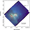 |
Fig. 1. Three-colour near-infrared image of Arp 220 obtained by combining NIRSpec narrow-band images tracing the continuum emission at ∼1 μm (blue), 3 μm (green), and 5 μm (red). The positions of the W and E nuclei are marked with crosses and match those of the nuclear parsec-scale disks observed in the millimeter with ALMA (Scoville et al. 2017). The box-circle symbol marks the position of the NE cluster. The cyan diamond indicates a region with fast multi-phase outflows (see Sect. 5.3). The NIRSpec angular resolution is of ∼2 − 3 spaxels (0.1−0.15″) in FWHM. |
The Arp 220 nuclear morphology is strongly affected by dust extinction, even in the NIR (see also Fig. A.1). The continuum emission appears as a crescent arc above the W nucleus at ∼1 μm and ∼3 μm. The E nucleus is barely visible at these wavelengths, but a few bright, clumpy regions likely associated with clusters can be identified (see also Scoville et al. 1998). The position of the brightest clump at ∼0.4″ (0.15 Kpc) north of the E nucleus is marked with a box-circle; hereinafter, we refer to it as the NE cluster, although it may be part of a more extended structure connecting the blue and green clumps in the regions between the nuclei in Fig. 1. The emission at ∼5 μm is mostly dominated by the two unresolved nuclei, which are marked in the figure with two crosses.
3.1. Spectral extraction
We extracted the spectra of the two nuclei and the NE cluster shown in Fig. 1 for each of the three NIRSpec gratings. We used apertures of three spaxels in radius, corresponding to 0.15″ or 55 pc. This aperture size broadly corresponds to two NIRSpec spatial resolution elements at 5 μm (FWHM ∼ 0.15″; D’Eugenio et al. 2023), thus ensuring that the entire point-source flux is captured at all wavelengths.
The three spectra are reported in Fig. 2. They are shown in rest frame, and their relative redshifts are taken into account: zW = 0.01774, zE = 0.01840, and zNE = 0.01870 (see Table 1). These values were obtained by measuring the centroid of the brightest hydrogen lines, and they are comparable with those inferred from sub-millimeter and millimeter ALMA spectroscopy at angular resolutions similar to those of NIRSpec (see Sect. 4.1).
 |
Fig. 2. Arp 220 NE cluster, W and E nuclear spectra from the three NIRSpec gratings. The spectra are shown in luminosity as a function of the rest frame wavelength. The vertical blue lines mark the positions of hydrogen transitions (dark to light blue indicate distinct hydrogen series). The orange lines identify H2 lines, the red lines are associated with [Fe II] transitions, and the green lines mark He I emission features. Strong broad-band absorption and emission features are also labelled in the figure. Zoom-in plots are presented in Appendix B. |
Properties of the Arp 220 nuclear regions.
The spectra show a few gaps in the wavelength coverage in the middle of the three bands. These result from the gap between the two NIRSpec detectors. The overlapping wavelength ranges at ∼1.85 μm and ∼3 μm perfectly match between the different bands, demonstrating a consistent flux calibration. We note that no aperture corrections were taken into account in this work.
3.2. Identification of the lines
The multitude of emission lines detected in NIRSpec spectra of Arp 220, which are marked in Fig. 2 with vertical lines, was identified using compilations of NIR features in star-forming and active galaxies from the literature (e.g. Lutz et al. 2000; Koo et al. 2016; Lamperti et al. 2017; Lee et al. 2017; Riffel et al. 2019). We also used the NIST atomic spectra database2 (Ralchenko 2005) and the high-resolution transmission molecular absorption database (HITRAN3, Rothman 2021) to provide probable identifications of faint lines that have not previously been reported in the literature.
Figures B.1–B.6 report all species we identified in the spectra of the Arp 220 nuclei and the NE cluster and compare them with those in the nuclear regions of another nearby interacting LIRG observed with NIRSpec, VV114 (e.g. Rich et al. 2023). Firmly detected line transitions are indicated with solid vertical lines, and they are also reported in Tables C.1, C.2, and C.3. Probable identifications are marked in the figures in the appendix with dotted vertical lines. All emission lines are well visible in the spectra of the south-west nucleus of VV114 (named SW-s2 by González-Alfonso et al. 2024) at a higher signal-to-noise ratio (S/N) and with narrower profiles than in Arp 220. All three nuclear regions of VV114, namely NE, SW-s1, and SW-s2, have been suggested to harbour deeply obscured AGN (e.g. Evans et al. 2022; Rich et al. 2023; Donnan et al. 2024; González-Alfonso et al. 20244). Hence, they serve as an optimal benchmark for a comparison with the nuclei of Arp 220, which are also thought to contain obscured AGN.
3.3. Modelling the continuum emission
To fit the stellar continuum, we used the penalised-pixel-fitting routine pPXF (Cappellari 2017). We used the MARCS synthetic library of stellar spectra to model the stellar continuum (Gustafsson et al. 2008). These templates have a constant spectral resolution λ/Δλ = 20 000 (σ ∼ 6 km s−1) and cover the range 0.13 − 20 μm with wavelengths in vacuum. Although not as reliable as an empirical stellar library, MARCS templates were preferred to E-MILES (Vazdekis et al. 2016), which have a lower spectral resolution than our NIRSpec data, and XSL (Verro et al. 2022), which have a narrower wavelength coverage and are affected by telluric features.
We also adopted a sixth-order multiplicative polynomial to better reproduce the continuum shape of the spectra. In addition, we used a set of gas emission line templates (parametrised with Gaussian profiles) together with the stellar templates to guide the fit. We fitted the band1 (0.95 − 1.86 μm) and band2 (1.63 − 3.11 μm) cubes separately, and the latter were restricted to wavelengths below 2.4 μm, corresponding to the cutoff of the detector gap. For band1, the wavelengths falling within the NIRSpec detector gap were appropriately masked during the fit procedure. The pPXF fit is likely to be degenerate in the linear combinations of stellar templates. However, this does not affect our goal. We do not require a realistic model of the star formation history and metallicity distribution; we only need an accurate stellar continuum model and a measurement of the stellar kinematics at the positions of the two nuclei.
Since no prominent stellar features are observed at wavelengths above 2.4 μm, and because of the dust emission and ice absorption (e.g. Donnan et al. 2024), we preferred to model the pseudo-continuum with a Savitzky–Golay filter after masking all prominent emission and absorption features.
In Figs. B.1–B.3 we report the reconstructed pPXF best-fit continuum emission, and Figs. B.4–B.6 show the pseudo-continuum shape in the two Arp 220 nuclei and the NE cluster. We used the (pseudo-)continuum-subtracted spectra to model the emission lines, and based on this, we derived the ISM kinematic and physical properties in these three regions.
3.4. Modelling the emission lines
After subtracting the (pseudo-)continuum, we modelled the most relevant gas emission lines using a combination of Gaussian profiles. In particular, we modelled a set of H I recombination lines, the Paschen (Pa), Brackett (Br), Pfund (Pf), and Humphreys (Hu) series, and molecular hydrogen features, as well as singly ionised iron transitions.
The sets of H I, H2 and [Fe II] transitions were modelled using independent fits to account for the fact that these three species can trace different gas phases and can therefore have different systemic velocities and line widths (e.g. May & Steiner 2017). All transitions were fitted using the Levenberg–Markwardt least-squares fitting code CAP-MPFIT (Cappellari 2017).
The transitions of a given species were fitted simultaneously (e.g. Perna et al. 2015) because this allows better constraints on the properties of the transitions associated with lower S/N. Namely, we constrained the wavelength separation between emission lines in accordance with atomic physics (considering their vacuum wavelengths). Moreover, we fixed their widths (in km s−1) so that they were the same for all the emission lines. Some emission lines are covered by two cubes (e.g. Brϵ at ∼1.82 μm, in band1 and band2 spectra). For these lines, we obtained an average profile by considering the errors from individual cubes as weights.
We performed two fits for each species, with one and two Gaussian components per emission line, respectively. The number of Gaussian sets (i.e. distinct kinematic components) we used to model the lines of a specific species was determined on the basis of the Bayesian information criterion (BIC; Schwarz 1978).
The measured fluxes of all identified emission line transitions are reported in Tables C.1, C.2, and C.3. To streamline the presentation, all tabulated fluxes were derived from single-Gaussian fits. A detailed Gaussian decomposition was instead used to infer the ISM properties discussed in Sect. 4. All line-width measurements reported in this manuscript were corrected for the instrumental broadening.
4. Results
In this section, we report the general characterisation of the nuclei and the NE cluster in terms of spectral shape, extinction, electron density, and the presence of outflows. These properties are discussed in Sect. 5 to investigate whether AGN signatures are present.
4.1. Systemic redshift of the two nuclei
We compared the three selected regions in Arp 220 after the individual spectra were reported in luminosity (λLλ) as a function of the rest-frame wavelength in vacuum. We used the centroid of the H I lines to determine the redshifts for the three spectra. These lines are quite symmetric and narrow and are therefore probably less affected by outflows and perturbed motions than other lines (see Perna et al. 2020; Wheeler et al. 2020). In contrast, the brightest H2 and [Fe II] lines show prominent blue wings and are blue-shifted by a few 10 s km s−1 with respect to the H I lines (Table 2).
Kinematic parameters.
The redshifts inferred from the atomic hydrogen lines are reported in Table 1. These values are consistent with those obtained from the stellar continuum modelling within the uncertainties (see Table 1). Moreover, our measurements match those obtained from the study of sub-millimeter and millimeter molecular line transitions, as reported in Sakamoto et al. (2021b), zW = 0.01762 and zE = 0.01802, and Pereira-Santaella et al. (2021), zW = 0.01760 and zE = 0.01792 (after reporting their radio velocities in barycentric reference frame for consistency with JWST data). In particular, for the W nucleus, all measurements are consistent within ∼30 km s−1. The molecular lines in the E nucleus are quite asymmetric (see Fig. 1 in Sakamoto et al. 2021b), resulting in slightly larger discrepancies compared to our NIR redshift. However, all measurements remain consistent within ≲100 km s−1, suggesting very little relative motion between the various components.
4.2. Qualitative comparison between the Arp 220 nuclear regions and the bright cluster
The spectra of the two nuclei and the NE cluster contain a high number of emission lines, which include the hydrogen lines (from the Pa, Br, Pf, and Hu series), as well as helium, iron, and the molecular hydrogen transitions. Notably, the H I lines appear to be a few times fainter in the E spectrum than in the W and NE spectra, probably because the extinction levels are higher (see Sect. 4.3) and the SFR is lower (Sect. 5.1). The W nucleus displays the most intense H2 lines, which are approximately twice stronger than those in the E and NE spectra. All emission lines appear to be narrow, although the brightest transitions show a moderate broadening and asymmetric profiles in the nuclei, which are signatures of outflows (see Sect. 4.5). No broad line region (BLR) emission line components (e.g. with FWHM > 1000 km s−1) are detected in any permitted emission line within the NIRSpec wavelength range.
At 3.3 μm, all three spectra show a broad emission feature that is produced by polycyclic aromatic hydrocarbons (PAHs). The 3.4 μm aliphatic features are also present in all three locations. PAHs and aliphatic transitions are stronger in the W nucleus by a factor of ∼3 (2) with respect to the E nucleus (NE cluster; see Sect. 5.1). This suggests that the SFR is higher in the W nucleus (as PAHs trace recent star formation activity; Sect. 5.1).
The prominent CO absorption bands at ∼1.6 μm and between 2.3 μm and 2.4 μm, produced in the atmospheres of giant and supergiant stars (Oliva et al. 1995) are clearly visible in the two nuclei as well as in the NE cluster.
Various other broad-band absorption features are visible as well, mostly produced by solid-state molecules of water ice (H2O, at 3 μm). These absorption features are stronger in the nuclear regions than in the nearby NE cluster. The 3.3 − 3.8 μm ice-band wing (Gibb et al. 2004) is prominent in the E nucleus and likely present in the W core. The strength of these absorption bands is therefore probably correlated with the abundance of dust, given that the two nuclear regions are most obscured in the millimeter range (Sakamoto et al. 2021a). Conversely, the carbon dioxide ice transitions 12CO2 at 4.27 μm and 13CO2 at 4.38 μm have rather peculiar shapes in the three spectra: the former is stronger in the E nucleus, but more asymmetric in the W nucleus (with a prominent blue shoulder), while the NE cluster shows an intermediate strength with respect to the nuclei. The 13CO2 is deeper and narrower in the W nucleus.
The W and E nuclei of Arp 220 show 12CO ro-vibrational lines up to Jlow = 23 (Fig. B.6), indicating the presence of high-excitation gas (lower-level energy of Elow = 1500 K). These transitions might provide a further indirect evidence of AGN activity. Detailed modelling is required to infer the CO gas properties and test the more likely mechanisms that cause this high excitation (e.g. Baba et al. 2022; González-Alfonso et al. 2024; Buiten et al. 2024; García-Bernete et al. 2024; Pereira-Santaella et al. 2024a). This analysis will be presented in a forthcoming paper (Buiten et al., in prep.).
The differences in the three spectra can also be appreciated from a qualitative comparison between their continuum shapes. From the shortest wavelengths to ∼1.8 μm, all three sources show a pronounced steepening in their spectra that is probably dominated by the diminishing effect of dust obscuration with increasing wavelength (see also Engel et al. 2011). In the range 1.8 − 2.3 μm, the W and NE spectra flatten, while the E spectrum still shows the same steepening observed at shortest wavelengths. This could suggest higher extinction at the position of the E nucleus as a result of the dust lane shown in reddish colours in Fig. 1. Between 2.3 and 5 μm, the nuclear regions show a mild increase in luminosity, but the NE cluster is almost constant. At ∼5 μm, the spectrum of the NE cluster reveals a modest rise in luminosity, while the two nuclei exhibit a much more pronounced increase that is probably caused by warm dust (Armus et al. 2007). It is therefore possible that dust-absorbed light is re-emitted at wavelengths ≳2 μm in the two nuclei. The higher dilution of CO bands at ∼2.3 − 2.4 μm in the nuclei compared to the NE cluster (Fig. B.3) also supports this possibility, as suggested by Engel et al. (2011).
In the next sections, we provide a concise quantitative overview of the general properties of some of these components. We do not pursue the full spectral energy distribution modelling further in this work, but instead use a subsequent paper to focus on a more detailed investigation.
4.3. Extinction
Extinction can have a strong effect on the estimated source luminosity and SFR. We therefore considered different methods for deriving its value. We compared pairs of emission lines at a wide wavelength separation for which the intrinsic ratio of the line strengths is known. We calculated the colour excess in terms of Paβ and Brγ,

where k is the value of the reddening curve evaluated at the Paβ and Brγ wavelengths, and the intrinsic ratio Paβ/Brγ was set to 5.88 assuming an electron temperature and a density of 104 K and 103 cm−3 (e.g. Osterbrock & Ferland 2006). We also used the Pfγ and Brδ to obtain an independent estimate for the colour excess,

where the intrinsic ratio Brδ/Pfγ was set to 1.71 (with the same assumptions as reported above). The coefficients in Eqs. (1) and (2) were derived assuming a Cardelli et al. (1989) extinction law.
We derived an additional estimate of the colour excess from the flux ratio of [Fe II] at 1.257 and 1.644 μm (e.g. Riffel et al. 2014), which are the two strongest iron lines in the NIR regime,
![$$ \begin{aligned} E(B-V) = 8.95 \log _{10} \left(\frac{1.34}{\left(\mathrm{[Fe\,II]}_{1.257}/\mathrm{[Fe\,II]}_{1.644}\right)_{\rm obs}}\right), \end{aligned} $$](/articles/aa/full_html/2024/10/aa50094-24/aa50094-24-eq55.gif)
where 1.34 is the intrinsic ratio (we note, however, that this is still a matter of some debate, and different values are reported in the literature, from 1.04 to 1.49; see Eriksen et al. 2009).
We measured a colour excess of the order of a few magnitudes (∼3 − 5) in the three regions of interest, corresponding to AV ∼ 10 − 14 (assuming RV = 3.1). We observed no significant differences in the measurements obtained from the three diagnostic ratios described above (Eqs. 1, 2, 3). Therefore, we refer below to the results obtained from Eq. 1. The most extreme extinction is associated with the E nucleus, with AV ∼ 14, consistent with the strongest steepening in the continuum emission at wavelengths ≲2 μm with respect to the W nucleus and the NE cluster (with AV ∼ 11, see Table 1). All measurements reported in this section were obtained for the narrow component of hydrogen and iron emission lines because the broad components are only well detected in the [Fe II] 1.644 μm and 1.257 μm pair of lines of the two nuclei. From these components, we obtained  (E) and 6 ± 1 (W), consistent with those obtained from the narrow-line components within 3σ.
In previous studies, an extinction of ≈6 mag in the innermost nuclear regions of Arp 220 was reported based on diagnostics such as the H I flux ratios Hα/Hβ (Perna et al. 2020), Hα/Paβ (Giménez-Arteaga et al. 2022), and Paα/Brγ (Engel et al. 2011). Slightly higher extinctions, AV ∼ 6 − 12, were measured from the K-band stellar continuum emission (Engel et al. 2011). More extreme values were obtained from mid-infrared diagnostics: For instance, Haas et al. (2001) reported an extinction of a few tens of magnitudes. This suggests that NIRSpec observations may only probe the outer gaseous layers, and that the total extinction towards the core of these dusty regions can be much higher than AV ∼ 10 − 14.
4.4. Electron density
We derived the electron density in the line-emitting regions surrounding the E, W, and NE regions of Arp 220 via the comparison of observed line strength ratios of [Fe II] transitions with theoretical values.
We used the ratio [Fe II] 1.677 μm/1.644 μm to infer electron densities in the range log (ne/cm−3) ≈3.5 − 4.5 for the three regions of interest (from Eq. 6 in Koo et al. 2016). For the two nuclei, for which two kinematic components are required to fit the total profiles, we considered the narrow components (because the broad component is not detected in the faint [Fe II] 1.677 μm). These measurements, reported in Table 1, are discussed in the context of previous measurements in Sect. 5.2.
4.5. Nuclear outflows
A distinctive feature of the Arp 220 nuclear environment are powerful and complex outflows. Compact and collimated cold molecular outflows, with velocities of a few 100 s km s−1, a bipolar morphology, and an extension of ∼120 pc are observed in both nuclei (e.g. Wheeler et al. 2020). Broader line profiles are instead observed in the ionised and neutral gas: For instance, Perna et al. (2021) reported W80 velocities (defined as the difference between the 90th and 10th percentile velocities of the fitted line profile) of ∼800 km s−1. However, these measurements were obtained from observations at lower spatial resolution (∼200 pc) and probably cannot be used to properly resolve the outflow kinematics on smaller scales.
Figure 3 shows the integrated spectra in the vicinity of the Paα (top), [Fe II] 1.644 μm (centre), and H2 2.12 μm (bottom) lines for the three regions of interest. The NE cluster shows symmetric and narrow profiles; conversely, broad and asymmetric (preferentially blue-shifted) line shapes are observed in the two nuclear regions, with outflowing gas at velocities up to −500 km s−1. We considered an outflow velocity of Vmax = |ΔVbroad|+2σbroad, where σbroad was corrected for the instrumental resolution (e.g. Fluetsch et al. 2021). In Table 2 we report the best-fit kinematic parameters and consider for the outflow velocities both non-parametric (e.g. W80, V10) and parametric measurements (e.g. Vmax) that are commonly used in the literature (see the caption of Table 2 for details).
 |
Fig. 3. Continuum-subtracted integrated spectra of the three regions of interest in the vicinity of the Paα, [Fe II] 1.644 μm, and H2 2.12 μm. The original spectra (in black) are reported in velocity space. The best-fit emission line profiles are shown in orange, and the individual Gaussian profiles used to reproduce the line shapes are reported in blue and green. Broad and asymmetric profiles are found in the nuclear spectra. The vertical lines mark the zero-velocity as inferred from the narrow component of the H I lines. The NIRSpec spectral resolution at the wavelengths of interest is σ ≈ 60 km s−1. |
A more detailed discussion of the AGN winds that might cause the broad and asymmetric profiles observed in the Arp 220 nuclei is presented in Sect. 5.3.
5. Discussion
We used the aperture-extracted spectra of the obscured nuclei E and W and the bright cluster NE to identify all gas emission line features in the NIRSpec spectral range, as well as the main absorption features due to ice and stars. We identified ∼70 atomic and ∼50 molecular emission lines. Tables C.1, C.2, and C.3 list the (vacuum) wavelengths and fluxes for all the firmly identified features in Arp 220, and Table 2 displays the kinematic parameters of the main optical lines discussed in this paper. We note that a few well-detected emission lines are not tabulated because (i) modelling them would require detailed deblending from other lines or (ii) their observed wavelengths are very close to the edges of the NIRSpec detector gaps.
In this section, we discuss the main features we observed in the spectra reported in Fig. 2 in relation with the possible presence of intense episodes of starburst activity and AGN accretion in the two nuclei.
5.1. Star formation tracers
We derived the instantaneous (∼10 Myr) SFR from the Paα dust-corrected luminosity following Giménez-Arteaga et al. (2022, and assuming a Chabrier 2003 initial mass function),
![$$ \begin{aligned} \mathrm{SFR}\,[M_\odot \,\mathrm{yr}^{-1}]&= 4.4\times 10^{-42} \times \left(\frac{\mathrm{H\alpha }}{\mathrm{Pa\alpha }}\right)_{\rm int} \times L(\mathrm{Pa\alpha })_{\rm corr}\,[\mathrm{erg\,s^{-1}}]\nonumber \\&= 3.7 \times 10^{-41} \times L(\mathrm{Pa}\alpha )_{\rm corr}\,[\mathrm{erg\,s^{-1}}], \end{aligned} $$](/articles/aa/full_html/2024/10/aa50094-24/aa50094-24-eq57.gif)
where the dust-corrected Paα luminosity can be obtained with A(Paα) = k(Paα) × E(B − V). In deriving Eq. (4), we assumed an electron density of 103 cm−3 (the dependence on ne is very weak) and temperature of 104 K. Moreover, for the E and W nuclear emission, we only considered the narrow components (dashed blue Gaussian lines in Fig. 3) and excluded the contribution of outflowing material in this way.
The use of E(B − V) inferred from Paβ/Brγ implies dust corrections of ∼5 − 8× factors for the Paα flux, resulting in an SFR ∼ 0.5 M⊙ yr−1 for the W nucleus, ∼0.2 M⊙ yr−1 for the E nucleus, and ∼0.9 M⊙ yr−1 for the NE cluster. Therefore, these three regions account for a total SFR(Paα) ∼2 M⊙ yr−1. For the extraction regions of ∼0.01 kpc2, these values would translate into star formation surface densities ΣSFR ∼ 20 − 100 M⊙ yr−1 kpc−2.
We also used the SFR calibration for the 3.3 μm PAH from Kim et al. (2012, see their Eq. 5) to convert the measured luminosities (L(PAH) = 2 × 1040 erg s−1 for the W, L(PAH) = 7 × 1039 erg s−1 for the E, and L(PAH) = 1040 erg s−1 for the NE cluster) into L(IR) and then the Kennicutt & Evans (2012)5 relation to derive dust-corrected SFR(PAH) in the range ∼1.5 − 3.4 M⊙ yr−1 (see Table 1). We note that the extinctions based on the recombination lines derived in Sect. 4.3 account for corrections of a factor of ∼2 at 3.3 μm.
In previous optical and NIR studies of Arp 220, slightly higher SFR measurements were obtained by integrating over the whole galaxy: Perna et al. (2020) reported an SFR(Hα)≲10 M⊙ yr−1 (using the Balmer decrement to correct for extinction), while Giménez-Arteaga et al. (2022) obtained an SFR(Paβ)∼19 M⊙ yr−1 from HST narrow-band images (using Paβ/Hα for the dust correction). Giménez-Arteaga et al. (2022) also reported the total SFR inferred from the 24 μm luminosity, 76 M⊙ yr−1. This value is significantly less affected by dust (AV ∼ 90 would imply a correction of a factor 2 at 24 μm). This value is more consistent with the total SFR(PAH) ∼ 40 M⊙ yr−1 we measure from NIRSpec data using an integrated spectrum extracted over a very large aperture (r = 1.5″, i.e. 0.56 kpc).
Therefore, our NIRSpec-based SFRs clearly agree with previous estimates obtained from optical, NIR, and mid-infrared bands. However, it is worth noting that the SFR inferred from the radio and millimeter regime appears to be several times higher, reaching 200–250 M⊙ yr−1 (e.g. Varenius et al. 2016; Pereira-Santaella et al. 2021). In particular, Varenius et al. (2016) and Pereira-Santaella et al. (2021) reported SFR ∼ 60 − 80 M⊙ yr−1 and ∼110 − 150 M⊙ yr−1 for the E and W nuclei separately, which is significantly higher than our NIR-based nuclear measurements. This discrepancy may stem from a combination of factors: (i) The far-IR and radio emission might not be attributable to star formation alone, but could also include contributions from AGN, which are entirely extinguished in the NIR. (ii) The SFR derived from FIR measurements traces the star formation history over a longer period (up to 100 Myr) than the Paα and PAH features (≲10 Myr). (iii) The total extinction towards the Arp 220 nuclear regions is much higher than AV ∼ 10 − 14 (e.g. Haas et al. 2001).
To summarise, the NIRSpec-based SFR measurements offer no solution to the existing discrepancy among various star formation tracers identified in previous studies.
5.2. High electron densities
The [Fe II]-based electron densities at the position of the two nuclei and the NE cluster (log(ne/cm−3)∼3.7 − 4.5) consistently exceed those inferred from optical [S II] 6718, 32 Å lines, which are of the order of 200 cm−3 (Perna et al. 2020). This suggests that the [Fe II] lines, having critical densities higher than [S II] (ncrit ∼ 1600 cm−3 for [S II] 6716 Å; ncrit ∼ 104 cm−3 for iron lines), trace post-shock regions with higher compression. An alternative explanation might be that the higher spatial resolution of NIRSpec data (∼0.1″ at the wavelengths of the ne-sensitive [Fe II] lines) compared to the MUSE observations (∼0.6″) enables a better isolation of the densest regions.
At higher redshift (up to z ∼ 9), the [S II] and [O II] 3727, 30 Å line ratios are systematically used to measure the ISM electron densities. Values in the range ∼300 − 1000 cm−3 are generally reported for AGN (e.g. Perna et al. 2017; Cresci et al. 2023) and star-forming galaxies (e.g. Förster Schreiber et al. 2019; Davies et al. 2021; Rodríguez Del Pino et al. 2024; Isobe et al. 2023; Lamperti et al. 2024). Significant correlations between ΣSFR and ne have been reported in the literature (e.g. Shimakawa et al. 2015), although they cover relatively narrow ranges in both ΣSFR (∼0.1–1 M⊙ yr−1 kpc−2) and ne(∼10 − 103 cm−3). From the extrapolation of these relations (e.g. Eq. 3 in Reddy et al. 2023) to the very high ΣSFR measured in Arp 220 (see Sect. 5.1), we would expect log(ne/cm−3)∼3. However, this value is roughly 30 times lower than the value measured at the position of the Arp 220 W nucleus using the [Fe II] lines. Instead, our measurements more closely resemble the electron densities observed in supernova remnants (e.g. Lee et al. 2017) and at the bases of protostar jets (e.g. Davis et al. 2011), with [Fe II]-based densities spanning log (ne/cm−3)≈3.5 − 4.5. Therefore, the extremely high [Fe II]-based electron densities we measured in the nuclei and the NE cluster could be due to higher levels of compression with respect to [S II] gas emitting in the optical.
We can definitely exclude any potential contamination from high-density AGN BLR in the [Fe II]-based electron densities obtained for the Arp 220 nuclei because the forbidden [Fe II] line transitions cannot originate from BLR high-density regions (Ne(BLR)≫Nc([Fe II])).
5.3. Multi-phase outflows
The NIRSpec nuclear spectra of Arp 220 show atomic and molecular gas transitions with broad profiles and prominent blue wings that are associated with outflows reaching velocities of up to Vmax ∼ 550 km s−1. In particular, high-velocity components are detected in Paα and [Fe II] 1.644 μm at the position of the E and W nuclei. Prominent H2 blue wings are solely observed in the E nucleus (Fig. 3). This suggests that the high-velocity gas in the W nucleus is sufficiently hot (because of shocks or intense ultraviolet radiation by hot stars or AGN) to disassociate the H2 molecules or, more in general, that different physical conditions may characterise its environment (e.g. in terms of the magnetic field and electron density in the outflowing gas; see e.g. Kristensen et al. 2023).
Nuclear outflows in the NIR H I, H2, and iron lines have been observed in nearby ULIRGs and active galaxies. While sources lacking an active SMBH typically exhibit less extreme outflow velocities (of about a few hundred km s−1), AGN can manifest outflows across a broad velocity range, from a few hundred to over a thousand km s−1 (e.g. Emonts et al. 2017; Perna et al. 2021; Speranza et al. 2022; Villar Martín et al. 2023). Consequently, it is challenging to distinguish between starburst- and AGN-driven outflows in Arp 220 based on velocity estimates alone. A more comprehensive analysis of the multi-phase and multi-scale outflows is necessary to elucidate whether the outflow energetics in Arp 220 are more consistent with AGN or starburst launching mechanisms. This work is presented in a companion paper (Ulivi et al. 2024).
We anticipate here that NIRSpec data show complex multiphase outflow structures that reach distances of ∼1 kpc and velocities of −900 km s−1 in the off-nuclear regions (Ulivi et al. 2024). Figure 4 shows the Paα and H2 2.12 μm line profiles extracted from a circular aperture of r = 0.15″ at a distance of ∼1.3″ to west of the W nucleus, as defined in Fig. 1 (cyan diamond). It corresponds to the base of the bright bubble visible in VLT SINFONI (Engel et al. 2011) and MUSE (Perna et al. 2020) observations, and shows the most extreme gas kinematics in the NIRSpec cube, with both ionised and molecular gas emission up to −900 km s−1 (Table 2). Similar velocities were also observed in the ionised and neutral gas phases at larger distances in the optical regime (e.g. Perna et al. 2020). A comprehensive characterisation of these outflows is required to better understand their origin.
 |
Fig. 4. Observed profiles of Paα and H2 2.12 μm, showing fast outflows. The spectra are extracted from the region in Fig. 1 marked with a cyan diamond, and they are reported in velocity space. The best-fit emission line profiles are shown in orange, and the individual Gaussian profiles used to reproduce the line shapes are reported in blue, purple, and green. The vertical grey lines mark the zero-velocity of the E nucleus, which is the most likely origin of the outflow shown in the figure (see the detailed discussion in Perna et al. 2020; Ulivi et al. 2024), and the dashed red vertical lines in the top panel identify the He I lines close to Paα (see Table C.1). |
5.4. Absence of high-ionisation lines
High-excitation emission lines with ionisation potentials IP > 54 eV (the He+ ionisation energy) can be formed either in gas that is photoionised by hard ultraviolet radiation or in very hot, collisionally ionised plasma. Therefore, they can be used as sign for AGN activity (e.g. Oliva et al. 1994; Moorwood et al. 1997).
Most of these highly ionised lines have previously been identified in ground-based (e.g. Rodríguez-Ardila et al. 2011; Lamperti et al. 2017; Cerqueira-Campos et al. 2021; den Brok et al. 2022) and space-based (e.g. Lutz et al. 2000; Sturm et al. 2002) NIR spectra of some nearby Seyfert galaxies (Table 3). No quantitative studies of the coronal lines prevalence in the AGN population have been conducted so far, but there are indications that these lines are more prevalent in unobscured type-1 sources rather than in obscured sources. This is consistent with the fact that some coronal lines have been recently detected with NIRSpec and MIRI in the nearby Seyfert 1.5 nucleus of NGC 7469 (Armus et al. 2023; Bianchin et al. 2024), but not in the highly obscured active nuclei of VV114 (see Appendix B; Donnan et al. 2024; González-Alfonso et al. 2024; Rich et al. 2023; but see also Speranza et al. 2022; Álvarez-Márquez et al. 2023). The lack of high-ionisation lines in AGN sources may reflect an AGN ionising continuum that lacks photons below a few keV. This could explain the absence of this line emission in obscured sources (e.g. Rodríguez-Ardila et al. 2011).
High-ionisation lines.
We searched for emission line features in the nuclear spectra of Arp 220 that might correspond to high-ionisation lines. We observed a bright feature near ∼4.488 μm, that is, close to the expected wavelength of the [Mg IV] line (IP ∼ 80 eV). Previous studies reported the detection of the [Mg IV] line in some nearby active galaxies together with other highly ionised species. For instance, Sturm et al. (2002) reported [Mg IV]/[Ar VI] ∼ 0.5 in Circinus and NGC 1068; Bianchin et al. (2024) obtained [Mg IV]/[Ar VI] ∼ 1.5 in NGC 7469. Notably, [Ar VI] is not detected in Arp 220. Because its IP is similar to that of [Mg IV] (see Table 3), the observed feature at the expected wavelength of [Mg IV] may involve alternative transitions. For instance, the low-ionisation line S I (λ4.4855 in vacuum, IP ∼ 10 eV) might cause the line features in the Arp 220 spectra.
Figure 5 shows the emission line at the wavelength position of the [Mg IV] in the three spectra of interest. These features are broad (FWHM ∼ 300 km s−1) and blue-shifted (ΔV ∼ −100 km s−1) with respect to the [Mg IV] expected wavelength (solid grey line at v = 0 km s−1). Moreover, their peaks are not at the systemic of the S I transition either. Pereira-Santaella et al. (2024b) recently reported a similar line in other nearby ULIRGs that do not host accreting SMBHs, with kinematic properties similar to those of Arp 220. The authors attributed this line to [Mg IV] and provided grids of photoionisation and shock models to determine the conditions under which [Mg IV] originates. Their analysis concluded that shocks from supernova explosions could explain the observed lines. In support of this scenario, we note that the line feature detected in Arp 220 is bright at the position of the blue and green clumps in the regions between the nuclei in Fig. 1, but it is faint in the surroundings of the two nuclei.
 |
Fig. 5. Continuum-subtracted integrated spectra of the three regions of interest in the vicinity of the [Mg IV] 4.488 μm. The original spectra (in black) are reported in velocity space. The best-fit emission line profiles are shown in orange. Broad and blueshifted profiles are found in the E nuclear spectrum. The vertical grey lines mark the zero-velocity as inferred from the narrow component of the H I lines, and the dashed red lines mark the expected position of the S I line. |
In Table 3, we report the main high-ionisation lines in the range covered by our NIRSpec spectra. For all but [Mg IV], we report the 3σ upper limits inferred from NIRSpec data. These upper limits, and in particular, the [Si VI] one, can be used to compare the NIRSpec measurements with those from the literature. In fact, [Si VI] is detected in a large number of AGN spectra (Lamperti et al. 2017; den Brok et al. 2022).
The top panel of Figure 6 shows the distribution of L([Si VI]) as a function of redshift for a sample of nearby active galaxies selected in the hard X-ray band (14−195 keV) from the Swift/Burst Alert Telescope (BAT) survey, as part of the BASS sample (Koss et al. 2017; Ricci et al. 2017). We display the [Si VI] detections and 3σ upper limits alongside the Arp 220 non-detections. It is evident that NIRSpec enables us to obtain more stringent upper limits compared to previous observations of other systems at z ∼ 0.018 (by ∼1 dex).
 |
Fig. 6. [Si VI] luminosity for Arp 220 and a sample of nearby AGN. Top panel: [Si VI] luminosity as a function of redshift for the sample of BASS AGN with detected (purple circles) and undetected (green squares) [Si VI] line from Lamperti et al. (2017). Arp 220 measurements are represented by red stars. For sources with undetected [Si VI] lines, we provide 3σ upper limits (illustrated with arrows). Bottom panel: [Si VI] luminosity as a function of intrinsic X-ray (2−10 keV) luminosity for the same sources as reported in the top panel. The dashed line indicate the linear relation between L([Si VI]) and L2 − 10 keV int obtained by Lamperti et al. (2017, not considering upper limits). X-ray luminosity upper limits for the nuclei of Arp 220 are taken from Paggi et al. (2017). |
The bottom panel of Figure 6 shows the correlation between intrinsic X-ray and [Si VI] luminosity (e.g. Rodríguez-Ardila et al. 2011; Lamperti et al. 2017) for the same sources. The upper limits for [Si VI] in Arp 220 nuclei are indicated at the intrinsic X-ray (2−10 keV) luminosities of < 1.4 × 1042 erg s−1 (W) and < 3.9 × 1042 erg s−1 (E), computed by Paggi et al. (2017) from the 3σ upper limits on the neutral Fe–Kα line. The Arp 220 [Si VI] upper limits are approximately 1 dex below the L([Si VI]) – L2 − 10 keV relation (dashed magenta line). However, it should be noted that measuring the intrinsic X-ray luminosity for highly obscured sources can be highly uncertain and that the Arp 220 X-ray luminosities are merely upper limits. Consequently, the nuclei of Arp 220 might not exhibit notable distinctions from other AGN with undetected [Si VI] reported in the figure, for which the presence of accreting SMBHs is confirmed in the hard X-ray band.
To conclude, no obvious highly ionised line emission is associated with AGN from either nucleus of Arp 220, even though the many bright H I, He I, H2, and low-excitation [Fe II] lines are detected at very high S/N. Moreover, the very stringent upper limits derived from NIRSpec observations cannot be used to discard the presence of AGN in Arp 220 nuclei when we take the extremely high nuclear extinction into account (Sect. 4.3).
5.5. Near-infrared emission-line diagnostic diagrams
We used the diagnostic diagrams presented by Riffel et al. (2013), Colina et al. (2015), and Calabrò et al. (2023) to investigate the ionisation mechanisms that cause the emission line ratios observed in the nuclei and the NE cluster. Prior to the analysis, all fluxes required for the diagnostics were corrected for dust extinction using the AV values reported in Table 1.
According to the diagram presented by Riffel et al. (2013), based on the H2 2.12 μm/Brγ versus [Fe II] 1.26 μm/Paβ line ratios, both nuclei and the NE cluster are in the AGN region. The NE cluster has slightly lower line ratios and it is therefore closer to the star-forming region in the diagram. In the diagram proposed by Colina et al. (2015), based on the H2 2.12 μm/Brγ versus [Fe II] 1.64 μm/Brγ, the two nuclei and NE cluster lie in the region that is dominated by AGN and supernovae. As the three regions show broadly similar line ratios, a similar ionisation mechanism should be present in the W, E, and NE regions of Arp 220, regardless of how the Riffel et al. (2013) and Colina et al. (2015) diagnostic diagrams are interpreted.
We also explored the diagnostic diagrams recently proposed by Calabrò et al. (2023), who used combinations of ratios of the [S III], [Fe II], [P II], and [C I] lines over hydrogen recombination lines. In all the diagrams, the two nuclei are slightly above the maximum starburst line (by 0.1−0.5 dex). The NE cluster lies on (or just below) the maximum starburst line. We note that the two nuclei are well above the maximum starburst line in the [C I]/Paβ diagram, which is compatible with both AGN and shock ionisations (see Fig. 13 in Calabrò et al. 2023).
In summary, these diagnostics do not allow us to distinguish between supernovae and AGN ionisation mechanisms. More detailed investigations of the flux ratios in the circumnuclear region of Arp 220 will be presented in a future work.
6. Conclusions
We provided an overview of the JWST/NIRSpec IFS observations of Arp 220. We introduced the data reduction and the continuum and emission line data modelling. We showed and discussed the near-infrared spectra of the E and W nuclei, together with the spectrum of a bright stellar cluster at ∼0.4″ (0.15 kpc) north-east from the E nucleus. These spectra were extracted using circular apertures of radius 55 pc (0.15″) for each region. In the following, we summarise our main findings.
We identified broadening and multiple kinematic components in the H I, H2 and [Fe II] lines caused by outflows (Fig. 3). The emission line features show maximum velocities of up to ∼550 km s−1 in the nuclear spectra. Even higher velocities (∼900 km s−1) are detected in the off-nuclear regions (Fig. 4). However, they do not conclusively represent direct evidence of AGN activity. Spatially resolved gas kinematics and outflow energetics, which will be used to test theoretical predictions for starburst- and AGN-driven winds, are discussed in a companion paper (Ulivi et al. 2024).
No high-ionisation lines associated with AGN activity were detected in the nuclear spectra of Arp 220. We observe the presence of bright [Mg IV] 4.488 μm lines (80 eV) in the two nuclear spectra and the NE stellar cluster (Fig. 5). However, no other high-ionisation lines are detected; in particular, the [Ar VI] 4.529 μm line, which has an IP and wavelength close to those of [Mg IV], is not detected. The [Mg IV] lines are broader (FWHM ∼ 300 km s−1) and more strongly blue-shifted (ΔV ∼ −100 km s−1) than the H I lines. Moreover, [Mg IV] is bright at the clusters positions, but it is faint in the surroundings of the two nuclei. These arguments suggest that this emission line is not produced by an AGN, but is instead due to stellar activity. This result is in line with recent findings of Pereira-Santaella et al. (2024b), who have reported [Mg IV] in other nearby ULIRGs that do not host accreting SMBHs, and associated [Mg IV] lines with shocks by supernova explosions.
The luminosity upper limits inferred for the high-ionisation (IP = 167 eV) [Si VI] emission line at the position of the Arp 220 nuclei are ∼1 dex below the L([Si VI])–L2 − 10 keV, int observed for X-ray AGN (Rodríguez-Ardila et al. 2011; Lamperti et al. 2017), but they are still broadly consistent with other sources hosting accreting SMBHs but lacking [Si VI] emission (Fig. 6).
We also reported high-excitation 12CO gas transitions (up to Jlow = 23) in the Arp 220 nuclei (Fig. B.6) that might be due to AGN activity (e.g. González-Alfonso et al. 2024). A companion paper (Buiten et al., in prep.) will provide detailed modelling of CO gas conditions to assess which mechanism, star formation and AGN, contributes to the observed high-excitation CO lines.
To conclude, an unambiguous identification of AGN in the Arp 220 system remains elusive after we studied the NIRSpec IFS nuclear spectra. At the same time, we cannot exclude accreting SMBHs because of the extreme extinction at the position of the two nuclei. The NIRSpec observations may only probe the outer gaseous layers, and the total extinction towards the core of the Arp 220 nuclear regions could be much higher than AV ∼ 11 − 14 based on recombination lines (see e.g. Haas et al. 2001; Sakamoto et al. 2021a). This might explain the absence of highly ionised gas transitions, as also reported in previous works on obscured AGN (e.g. Rodríguez-Ardila et al. 2011; Lamperti et al. 2017).
Slightly smaller (but consistent) values would be obtained using the Piqueras López et al. (2016) relation.
Acknowledgments
We thank the anonymous referee for useful comments. We are grateful to Paul van der Werf, Victorine Buiten, and Angèle Taillard for discussing various aspects of this work. MP, SA, and BRP acknowledge support from the research project PID2021-127718NB-I00 of the Spanish Ministry of Science and Innovation/State Agency of Research (MCIN/AEI/10.13039/501100011033). IL acknowledges support from PID2022-140483NB-C22 funded by AEI 10.13039/501100011033 and BDC 20221289 funded by MCIN by the Recovery, Transformation and Resilience Plan from the Spanish State, and by NextGenerationEU from the European Union through the Recovery and Resilience Facility. MPS acknowledges support from grants RYC2021-033094-I and CNS2023-145506 funded by MCIN/AEI/10.13039/501100011033 and the European Union NextGenerationEU/PRTR. RM acknowledges support by the Science and Technology Facilities Council (STFC), by the ERC Advanced Grant 695671 “QUENCH”, and by the UKRI Frontier Research grant RISEandFALL; RM is further supported by a research professorship from the Royal Society. AJB acknowledges funding from the “First Galaxies” Advanced Grant from the European Research Council (ERC) under the European Union’s Horizon 2020 research and innovation program (Grant agreement No. 789056). GC, MP, and LU acknowledge the support of the INAF Large Grant 2022 “The metal circle: a new sharp view of the baryon cycle up to Cosmic Dawn with the latest generation IFU facilities”. HÜ gratefully acknowledges support by the Isaac Newton Trust and by the Kavli Foundation through a Newton-Kavli Junior Fellowship.
References
- Álvarez-Márquez, J., Labiano, A., Guillard, P., et al. 2023, A&A, 672, A108 [NASA ADS] [CrossRef] [EDP Sciences] [Google Scholar]
- Armus, L., Charmandaris, V., Bernard-Salas, J., et al. 2007, ApJ, 656, 148 [NASA ADS] [CrossRef] [Google Scholar]
- Armus, L., Lai, T., U, V., et al. 2023, ApJ, 942, L37 [NASA ADS] [CrossRef] [Google Scholar]
- Arp, H. 1966, ApJS, 14, 1 [NASA ADS] [CrossRef] [Google Scholar]
- Arribas, S., Colina, L., & Clements, D. 2001, ApJ, 560, 160 [Google Scholar]
- Baan, W. A., & Haschick, A. D. 1995, ApJ, 454, 745 [NASA ADS] [CrossRef] [Google Scholar]
- Baba, S., Imanishi, M., Izumi, T., et al. 2022, ApJ, 928, 184 [NASA ADS] [CrossRef] [Google Scholar]
- Barcos-Muñoz, L., Leroy, A. K., Evans, A. S., et al. 2015, ApJ, 799, 10 [Google Scholar]
- Bennett, C. L., Larson, D., Weiland, J. L., & Hinshaw, G. 2014, ApJ, 794, 135 [Google Scholar]
- Bianchin, M., U, V., Song, Y., et al. 2024, ApJ, 965, 103 [NASA ADS] [CrossRef] [Google Scholar]
- Böker, T., Arribas, S., Lützgendorf, N., et al. 2022, A&A, 661, A82 [NASA ADS] [CrossRef] [EDP Sciences] [Google Scholar]
- Böker, T., Beck, T. L., Birkmann, S. M., et al. 2023, PASP, 135, 038001 [CrossRef] [Google Scholar]
- Buiten, V. A., van der Werf, P. P., Viti, S., et al. 2024, ApJ, 966, 166 [NASA ADS] [CrossRef] [Google Scholar]
- Calabrò, A., Pentericci, L., Feltre, A., et al. 2023, A&A, 679, A80 [NASA ADS] [CrossRef] [EDP Sciences] [Google Scholar]
- Cappellari, M. 2017, MNRAS, 466, 798 [Google Scholar]
- Cardelli, J. A., Clayton, G. C., & Mathis, J. S. 1989, ApJ, 345, 245 [Google Scholar]
- Cerqueira-Campos, F. C., Rodríguez-Ardila, A., Riffel, R., et al. 2021, MNRAS, 500, 2666 [Google Scholar]
- Chabrier, G. 2003, PASP, 115, 763 [Google Scholar]
- Chandar, R., Caputo, M., Linden, S., et al. 2023, ApJ, 943, 142 [NASA ADS] [CrossRef] [Google Scholar]
- Colina, L., Arribas, S., & Clements, D. 2004, ApJ, 602, 181 [Google Scholar]
- Colina, L., Piqueras López, J., Arribas, S., et al. 2015, A&A, 578, A48 [NASA ADS] [CrossRef] [EDP Sciences] [Google Scholar]
- Cresci, G., Tozzi, G., Perna, M., et al. 2023, A&A, 672, A128 [NASA ADS] [CrossRef] [EDP Sciences] [Google Scholar]
- Davies, R. L., Förster Schreiber, N. M., Genzel, R., et al. 2021, ApJ, 909, 78 [NASA ADS] [CrossRef] [Google Scholar]
- Davis, C. J., Cervantes, B., Nisini, B., et al. 2011, A&A, 528, A3 [NASA ADS] [CrossRef] [EDP Sciences] [Google Scholar]
- den Brok, J. S., Koss, M. J., Trakhtenbrot, B., et al. 2022, ApJS, 261, 7 [NASA ADS] [CrossRef] [Google Scholar]
- D’Eugenio, F., Perez-Gonzalez, P., Maiolino, R., et al. 2023, ArXiv e-prints [arXiv:2308.06317] [Google Scholar]
- Donnan, F. R., García-Bernete, I., Rigopoulou, D., et al. 2024, MNRAS, 529, 1386 [NASA ADS] [CrossRef] [Google Scholar]
- Emonts, B. H. C., Colina, L., Piqueras-López, J., et al. 2017, A&A, 607, A116 [NASA ADS] [CrossRef] [EDP Sciences] [Google Scholar]
- Engel, H., Davies, R. I., Genzel, R., et al. 2011, ApJ, 729, 58 [NASA ADS] [CrossRef] [Google Scholar]
- Eriksen, K. A., Arnett, D., McCarthy, D. W., & Young, P. 2009, ApJ, 697, 29 [CrossRef] [Google Scholar]
- Evans, A. S., Frayer, D. T., Charmandaris, V., et al. 2022, ApJ, 940, L8 [NASA ADS] [CrossRef] [Google Scholar]
- Fluetsch, A., Maiolino, R., Carniani, S., et al. 2021, MNRAS, 505, 5753 [NASA ADS] [CrossRef] [Google Scholar]
- Förster Schreiber, N. M., Übler, H., Davies, R. L., et al. 2019, ApJ, 875, 21 [Google Scholar]
- García-Bernete, I., Pereira-Santaella, M., González-Alfonso, E., et al. 2024, A&A, 682, L5 [NASA ADS] [CrossRef] [EDP Sciences] [Google Scholar]
- Gibb, E. L., Whittet, D. C. B., Boogert, A. C. A., & Tielens, A. G. G. M. 2004, ApJS, 151, 35 [NASA ADS] [CrossRef] [Google Scholar]
- Giménez-Arteaga, C., Brammer, G. B., Marchesini, D., et al. 2022, ApJS, 263, 17 [CrossRef] [Google Scholar]
- González-Alfonso, E., García-Bernete, I., Pereira-Santaella, M., et al. 2024, A&A, 682, A182 [NASA ADS] [CrossRef] [EDP Sciences] [Google Scholar]
- Gustafsson, B., Edvardsson, B., Eriksson, K., et al. 2008, A&A, 486, 951 [NASA ADS] [CrossRef] [EDP Sciences] [Google Scholar]
- Haas, M., Klaas, U., Müller, S. A. H., Chini, R., & Coulson, I. 2001, A&A, 367, L9 [NASA ADS] [CrossRef] [EDP Sciences] [Google Scholar]
- Isobe, Y., Ouchi, M., Nakajima, K., et al. 2023, ApJ, 956, 139 [NASA ADS] [CrossRef] [Google Scholar]
- Jakobsen, P., Ferruit, P., de Oliveira, C. A., et al. 2022, A&A, 661, A80 [NASA ADS] [CrossRef] [EDP Sciences] [Google Scholar]
- Kennicutt, R. C., & Evans, N. J. 2012, ARA&A, 50, 531 [NASA ADS] [CrossRef] [Google Scholar]
- Kim, J. H., Im, M., Lee, H. M., et al. 2012, ApJ, 760, 120 [NASA ADS] [CrossRef] [Google Scholar]
- Koo, B.-C., Raymond, J. C., & Kim, H.-J. 2016, J. Korean Astron. Soc., 49, 109 [NASA ADS] [CrossRef] [Google Scholar]
- Koss, M., Trakhtenbrot, B., Ricci, C., et al. 2017, ApJ, 850, 74 [Google Scholar]
- Kristensen, L. E., Godard, B., Guillard, P., Gusdorf, A., & Pineau des Forêts, G. 2023, A&A, 675, A86 [NASA ADS] [CrossRef] [EDP Sciences] [Google Scholar]
- Lamperti, I., Koss, M., Trakhtenbrot, B., et al. 2017, MNRAS, 467, 540 [Google Scholar]
- Lamperti, I., Pereira-Santaella, M., Perna, M., et al. 2022, A&A, 668, A45 [NASA ADS] [CrossRef] [EDP Sciences] [Google Scholar]
- Lamperti, I., Arribas, S., Perna, M., et al. 2024, A&A, in press, https://doi.org/10.1051/0004-6361/202451021 [Google Scholar]
- Law, D. D., Morrison, J. E., Argyriou, I., et al. 2023, AJ, 166, 45 [NASA ADS] [CrossRef] [Google Scholar]
- Lee, Y.-H., Koo, B.-C., Moon, D.-S., Burton, M. G., & Lee, J.-J. 2017, ApJ, 837, 118 [NASA ADS] [CrossRef] [Google Scholar]
- Lockhart, K. E., Kewley, L. J., Lu, J. R., et al. 2015, ApJ, 810, 149 [CrossRef] [Google Scholar]
- Lutz, D., Sturm, E., Genzel, R., et al. 2000, ApJ, 536, 697 [CrossRef] [Google Scholar]
- May, D., & Steiner, J. E. 2017, MNRAS, 469, 994 [NASA ADS] [CrossRef] [Google Scholar]
- McDowell, J. C., Clements, D. L., Lamb, S. A., et al. 2003, ApJ, 591, 154 [NASA ADS] [CrossRef] [Google Scholar]
- Moorwood, A. F. M., Marconi, A., van der Werf, P. P., & Oliva, E. 1997, Ap&SS, 248, 113 [NASA ADS] [CrossRef] [Google Scholar]
- Nardini, E., Risaliti, G., Watabe, Y., Salvati, M., & Sani, E. 2010, MNRAS, 405, 2505 [NASA ADS] [Google Scholar]
- Oliva, E., Salvati, M., Moorwood, A. F. M., & Marconi, A. 1994, A&A, 288, 457 [NASA ADS] [Google Scholar]
- Oliva, E., Origlia, L., Kotilainen, J. K., & Moorwood, A. F. M. 1995, A&A, 301, 55 [NASA ADS] [Google Scholar]
- Osterbrock, D. E., & Ferland, G. J. 2006, Astrophysics of Gaseous Nebulae and Active Galactic Nuclei (Sausalito: University Science Books) [Google Scholar]
- Paggi, A., Fabbiano, G., Risaliti, G., et al. 2017, ApJ, 841, 44 [NASA ADS] [CrossRef] [Google Scholar]
- Pereira-Santaella, M., Colina, L., García-Burillo, S., et al. 2021, A&A, 651, A42 [NASA ADS] [CrossRef] [EDP Sciences] [Google Scholar]
- Pereira-Santaella, M., González-Alfonso, E., García-Bernete, I., García-Burillo, S., & Rigopoulou, D. 2024a, A&A, 681, A117 [NASA ADS] [CrossRef] [EDP Sciences] [Google Scholar]
- Pereira-Santaella, M., García-Bernete, I., González-Alfonso, E., et al. 2024b, A&A, 685, L13 [NASA ADS] [CrossRef] [EDP Sciences] [Google Scholar]
- Perna, M., Brusa, M., Cresci, G., et al. 2015, A&A, 574, A82 [NASA ADS] [CrossRef] [EDP Sciences] [Google Scholar]
- Perna, M., Lanzuisi, G., Brusa, M., Cresci, G., & Mignoli, M. 2017, A&A, 606, A96 [NASA ADS] [CrossRef] [EDP Sciences] [Google Scholar]
- Perna, M., Arribas, S., Catalán-Torrecilla, C., et al. 2020, A&A, 643, A139 [NASA ADS] [CrossRef] [EDP Sciences] [Google Scholar]
- Perna, M., Arribas, S., Pereira Santaella, M., et al. 2021, A&A, 646, A101 [EDP Sciences] [Google Scholar]
- Perna, M., Arribas, S., Marshall, M., et al. 2023, A&A, 679, A89 [NASA ADS] [CrossRef] [EDP Sciences] [Google Scholar]
- Piqueras López, J., Colina, L., Arribas, S., Pereira-Santaella, M., & Alonso-Herrero, A. 2016, A&A, 590, A67 [NASA ADS] [CrossRef] [EDP Sciences] [Google Scholar]
- Ralchenko, Y. 2005, Mem. Soc. Astron. It. Suppl., 8, 96 [Google Scholar]
- Reddy, N. A., Sanders, R. L., Shapley, A. E., et al. 2023, ApJ, 951, 56 [NASA ADS] [CrossRef] [Google Scholar]
- Ricci, C., Trakhtenbrot, B., Koss, M. J., et al. 2017, ApJS, 233, 17 [Google Scholar]
- Rich, J., Aalto, S., Evans, A. S., et al. 2023, ApJ, 944, L50 [CrossRef] [Google Scholar]
- Riffel, R., Rodríguez-Ardila, A., Aleman, I., et al. 2013, MNRAS, 430, 2002 [NASA ADS] [CrossRef] [Google Scholar]
- Riffel, R. A., Vale, T. B., Storchi-Bergmann, T., & McGregor, P. J. 2014, MNRAS, 442, 656 [NASA ADS] [CrossRef] [Google Scholar]
- Riffel, R., Rodríguez-Ardila, A., Brotherton, M. S., et al. 2019, MNRAS, 486, 3228 [Google Scholar]
- Rodríguez-Ardila, A., Prieto, M. A., Portilla, J. G., & Tejeiro, J. M. 2011, ApJ, 743, 100 [Google Scholar]
- Rodríguez Del Pino, B., Perna, M., Arribas, S., et al. 2024, A&A, 684, A187 [NASA ADS] [CrossRef] [EDP Sciences] [Google Scholar]
- Rothman, L. S. 2021, Nat. Rev. Phys., 3, 302 [CrossRef] [Google Scholar]
- Sakamoto, K., González-Alfonso, E., Martín, S., et al. 2021a, ApJ, 923, 206 [NASA ADS] [CrossRef] [Google Scholar]
- Sakamoto, K., Martín, S., Wilner, D. J., et al. 2021b, ApJ, 923, 240 [NASA ADS] [CrossRef] [Google Scholar]
- Schwarz, U. J. 1978, A&A, 65, 345 [NASA ADS] [Google Scholar]
- Scoville, N. Z., Evans, A. S., Dinshaw, N., et al. 1998, ApJ, 492, L107 [NASA ADS] [CrossRef] [Google Scholar]
- Scoville, N., Aussel, H., Brusa, M., et al. 2007, ApJS, 172, 1 [Google Scholar]
- Scoville, N., Murchikova, L., Walter, F., et al. 2017, ApJ, 836, 66 [Google Scholar]
- Shimakawa, R., Kodama, T., Steidel, C. C., et al. 2015, MNRAS, 451, 1284 [Google Scholar]
- Speranza, G., Ramos Almeida, C., Acosta-Pulido, J. A., et al. 2022, A&A, 665, A55 [NASA ADS] [CrossRef] [EDP Sciences] [Google Scholar]
- Sturm, E., Lutz, D., Verma, A., et al. 2002, A&A, 393, 821 [NASA ADS] [CrossRef] [EDP Sciences] [Google Scholar]
- Teng, S. H., Rigby, J. R., Stern, D., et al. 2015, ApJ, 814, 56 [Google Scholar]
- Ueda, J., Michiyama, T., Iono, D., Miyamoto, Y., & Saito, T. 2022, PASJ, 74, 407 [NASA ADS] [CrossRef] [Google Scholar]
- Ulivi, L., Perna, M., Lamperti, I., et al. 2024, A&A, submitted [arXiv:2407.08505] [Google Scholar]
- Varenius, E., Conway, J. E., Martí-Vidal, I., et al. 2016, A&A, 593, A86 [NASA ADS] [CrossRef] [EDP Sciences] [Google Scholar]
- Varenius, E., Conway, J. E., Batejat, F., et al. 2019, A&A, 623, A173 [NASA ADS] [CrossRef] [EDP Sciences] [Google Scholar]
- Vazdekis, A., Koleva, M., Ricciardelli, E., Röck, B., & Falcón-Barroso, J. 2016, MNRAS, 463, 3409 [Google Scholar]
- Verro, K., Trager, S. C., Peletier, R. F., et al. 2022, A&A, 660, A34 [NASA ADS] [CrossRef] [EDP Sciences] [Google Scholar]
- Villar Martín, M., Castro-Rodríguez, N., Pereira Santaella, M., et al. 2023, A&A, 673, A25 [NASA ADS] [CrossRef] [EDP Sciences] [Google Scholar]
- Wheeler, J., Glenn, J., Rangwala, N., & Fyhrie, A. 2020, ApJ, 896, 43 [NASA ADS] [CrossRef] [Google Scholar]
- Yoast-Hull, T. M., & Murray, N. 2019, MNRAS, 484, 3665 [NASA ADS] [CrossRef] [Google Scholar]
- Yoast-Hull, T. M., Gallagher, J. S., Aalto, S., & Varenius, E. 2017, MNRAS, 469, L89 [NASA ADS] [CrossRef] [Google Scholar]
Appendix A: NIRSpec narrow-band images
 |
Fig. A.1. NIRSpec narrow-band images tracing the continuum emission at ∼1 μm (top), 3 μm (centre) and 5 μm (bottom). The position of the W and E nuclei are marked with X symbols; the box-circle symbol marks the position of the bright NE cluster (see also Fig. 1) |
Appendix B: Integrated spectra
 |
Fig. B.1. 0.95 − 1.42 μm portion on the spectra of the Arp 220 and VV114 nuclear regions. The spectra are shown in luminosity as a function of the rest frame wavelength, considering the redshift of each region. The grey, cyan and orange curves represent the pPXF best-fit. The vertical blue lines mark the position of hydrogen transitions; the orange lines identify H2 lines; the red lines are associated with [Fe II] transitions; the green lines mark He I features; solid vertical lines mark the position of faint metal lines; potential identifications are indicated with dotted vertical lines. The positions of highly ionised gas transitions are indicated with narrow vertical bands in purple. In the figure, we also indicate the position of strong stellar absorption features. |
 |
Fig. B.2. 1.45 − 1.86 μm portion on the spectra of the Arp 220 and VV114 nuclear regions. See B.1 for details. We note that at ∼1.715 μm there is an overlap of two vertical lines, associated with the detected H2 1.7149 μm (in orange) and the undetected [Ti VI] 1.7156 μm (in purple). |
 |
Fig. B.3. 1.85 − 2.40 μm portion on the spectra of the Arp 220 and VV114 nuclear regions. See B.1 for further details. |
 |
Fig. B.4. 2.4 − 3.1 μm portion on the spectra of the Arp 220 and VV114 nuclear regions. The pseudo-continuum described in Sect. 3.3 are shown with dashed curves. See B.1 for further details. |
 |
Fig. B.5. 3.1 − 4.0 μm portion on the spectra of the Arp 220 and VV114 nuclear regions. See B.1 for further details. |
 |
Fig. B.6. 4.1 − 5.2 μm portion on the spectra of Arp 220 and VV114 nuclear regions. The E and W nuclei show 12CO ro-vibrational lines up to Jlow = 23 (i.e. within the wavelength range marked with a dot-dashed horizontal line; for completeness, 13CO range is also reported, similar to Fig. 2 in González-Alfonso et al. 2024). Detailed modelling of the CO transitions will be presented in Buiten et al., in prep. See B.1 for further details. |
Appendix C: Arp 220 emission line lists
Arp 220 emission line list in the W and E nuclei, and NE cluster (band1 spectra)
Arp 220 emission line list in the W and E nuclei, and NE cluster (band2 spectra)
Arp 220 emission line list in the W and E nuclei, and NE cluster (band3 spectra)
All Tables
Arp 220 emission line list in the W and E nuclei, and NE cluster (band1 spectra)
Arp 220 emission line list in the W and E nuclei, and NE cluster (band2 spectra)
Arp 220 emission line list in the W and E nuclei, and NE cluster (band3 spectra)
All Figures
|
Fig. 1. Three-colour near-infrared image of Arp 220 obtained by combining NIRSpec narrow-band images tracing the continuum emission at ∼1 μm (blue), 3 μm (green), and 5 μm (red). The positions of the W and E nuclei are marked with crosses and match those of the nuclear parsec-scale disks observed in the millimeter with ALMA (Scoville et al. 2017). The box-circle symbol marks the position of the NE cluster. The cyan diamond indicates a region with fast multi-phase outflows (see Sect. 5.3). The NIRSpec angular resolution is of ∼2 − 3 spaxels (0.1−0.15″) in FWHM. |
| In the text | |
|
Fig. 2. Arp 220 NE cluster, W and E nuclear spectra from the three NIRSpec gratings. The spectra are shown in luminosity as a function of the rest frame wavelength. The vertical blue lines mark the positions of hydrogen transitions (dark to light blue indicate distinct hydrogen series). The orange lines identify H2 lines, the red lines are associated with [Fe II] transitions, and the green lines mark He I emission features. Strong broad-band absorption and emission features are also labelled in the figure. Zoom-in plots are presented in Appendix B. |
| In the text | |
|
Fig. 3. Continuum-subtracted integrated spectra of the three regions of interest in the vicinity of the Paα, [Fe II] 1.644 μm, and H2 2.12 μm. The original spectra (in black) are reported in velocity space. The best-fit emission line profiles are shown in orange, and the individual Gaussian profiles used to reproduce the line shapes are reported in blue and green. Broad and asymmetric profiles are found in the nuclear spectra. The vertical lines mark the zero-velocity as inferred from the narrow component of the H I lines. The NIRSpec spectral resolution at the wavelengths of interest is σ ≈ 60 km s−1. |
| In the text | |
|
Fig. 4. Observed profiles of Paα and H2 2.12 μm, showing fast outflows. The spectra are extracted from the region in Fig. 1 marked with a cyan diamond, and they are reported in velocity space. The best-fit emission line profiles are shown in orange, and the individual Gaussian profiles used to reproduce the line shapes are reported in blue, purple, and green. The vertical grey lines mark the zero-velocity of the E nucleus, which is the most likely origin of the outflow shown in the figure (see the detailed discussion in Perna et al. 2020; Ulivi et al. 2024), and the dashed red vertical lines in the top panel identify the He I lines close to Paα (see Table C.1). |
| In the text | |
|
Fig. 5. Continuum-subtracted integrated spectra of the three regions of interest in the vicinity of the [Mg IV] 4.488 μm. The original spectra (in black) are reported in velocity space. The best-fit emission line profiles are shown in orange. Broad and blueshifted profiles are found in the E nuclear spectrum. The vertical grey lines mark the zero-velocity as inferred from the narrow component of the H I lines, and the dashed red lines mark the expected position of the S I line. |
| In the text | |
|
Fig. 6. [Si VI] luminosity for Arp 220 and a sample of nearby AGN. Top panel: [Si VI] luminosity as a function of redshift for the sample of BASS AGN with detected (purple circles) and undetected (green squares) [Si VI] line from Lamperti et al. (2017). Arp 220 measurements are represented by red stars. For sources with undetected [Si VI] lines, we provide 3σ upper limits (illustrated with arrows). Bottom panel: [Si VI] luminosity as a function of intrinsic X-ray (2−10 keV) luminosity for the same sources as reported in the top panel. The dashed line indicate the linear relation between L([Si VI]) and L2 − 10 keV int obtained by Lamperti et al. (2017, not considering upper limits). X-ray luminosity upper limits for the nuclei of Arp 220 are taken from Paggi et al. (2017). |
| In the text | |
|
Fig. A.1. NIRSpec narrow-band images tracing the continuum emission at ∼1 μm (top), 3 μm (centre) and 5 μm (bottom). The position of the W and E nuclei are marked with X symbols; the box-circle symbol marks the position of the bright NE cluster (see also Fig. 1) |
| In the text | |
|
Fig. B.1. 0.95 − 1.42 μm portion on the spectra of the Arp 220 and VV114 nuclear regions. The spectra are shown in luminosity as a function of the rest frame wavelength, considering the redshift of each region. The grey, cyan and orange curves represent the pPXF best-fit. The vertical blue lines mark the position of hydrogen transitions; the orange lines identify H2 lines; the red lines are associated with [Fe II] transitions; the green lines mark He I features; solid vertical lines mark the position of faint metal lines; potential identifications are indicated with dotted vertical lines. The positions of highly ionised gas transitions are indicated with narrow vertical bands in purple. In the figure, we also indicate the position of strong stellar absorption features. |
| In the text | |
|
Fig. B.2. 1.45 − 1.86 μm portion on the spectra of the Arp 220 and VV114 nuclear regions. See B.1 for details. We note that at ∼1.715 μm there is an overlap of two vertical lines, associated with the detected H2 1.7149 μm (in orange) and the undetected [Ti VI] 1.7156 μm (in purple). |
| In the text | |
|
Fig. B.3. 1.85 − 2.40 μm portion on the spectra of the Arp 220 and VV114 nuclear regions. See B.1 for further details. |
| In the text | |
|
Fig. B.4. 2.4 − 3.1 μm portion on the spectra of the Arp 220 and VV114 nuclear regions. The pseudo-continuum described in Sect. 3.3 are shown with dashed curves. See B.1 for further details. |
| In the text | |
|
Fig. B.5. 3.1 − 4.0 μm portion on the spectra of the Arp 220 and VV114 nuclear regions. See B.1 for further details. |
| In the text | |
|
Fig. B.6. 4.1 − 5.2 μm portion on the spectra of Arp 220 and VV114 nuclear regions. The E and W nuclei show 12CO ro-vibrational lines up to Jlow = 23 (i.e. within the wavelength range marked with a dot-dashed horizontal line; for completeness, 13CO range is also reported, similar to Fig. 2 in González-Alfonso et al. 2024). Detailed modelling of the CO transitions will be presented in Buiten et al., in prep. See B.1 for further details. |
| In the text | |
Current usage metrics show cumulative count of Article Views (full-text article views including HTML views, PDF and ePub downloads, according to the available data) and Abstracts Views on Vision4Press platform.
Data correspond to usage on the plateform after 2015. The current usage metrics is available 48-96 hours after online publication and is updated daily on week days.
Initial download of the metrics may take a while.