| Issue |
A&A
Volume 690, October 2024
|
|
|---|---|---|
| Article Number | A282 | |
| Number of page(s) | 10 | |
| Section | Stellar structure and evolution | |
| DOI | https://doi.org/10.1051/0004-6361/202450353 | |
| Published online | 17 October 2024 | |
Analytic approximations for massive close post-mass transfer binary systems
1
Argelander-Institut für Astronomie, Universität Bonn, Auf dem Hügel 71, 53121 Bonn, Germany
2
Max-Planck-Institut für Radioastronomie, Auf dem Hügel 69, 53121 Bonn, Germany
3
Instituut voor Sterrenkunde, KU Leuven, Celestijnenlaan 200D, 3001 Leuven, Belgium
4
Max Planck-Institut für Astrophysik, Karl-Schwarzschild-Straße 1, 85748 Garching, Germany
5
Institute of Astronomy, Faculty of Physics, Astronomy and Informatics, Nicolaus Copernicus University, Grudziadzka 5, 87-100 Toruń, Poland
Received:
12
April
2024
Accepted:
18
July
2024
Massive binary evolution models are needed to predict massive star populations in star-forming galaxies, the supernova diversity, and the number and properties of gravitational wave sources. Such models are often computed using so-called rapid binary evolution codes, which approximate the evolution of the binary components based on detailed single star models. However, about one-third of the interacting massive binary stars undergo mass transfer during core hydrogen-burning (Case A mass transfer), whose outcome is difficult to derive from single star models. For this work, we used a large grid of detailed binary evolution models for primaries in the initial mass range 10–40 M⊙ with a Large and Small Magellanic Cloud composition, to derive analytic fits for the key quantities needed in rapid binary evolution codes, that is, the duration of core hydrogen-burning, and the resulting donor star mass. We find that systems with shorter orbital periods produce up to 50% lighter stripped donors and have a lifetime up to 30% larger than wider systems. Both quantities strongly depend on the initial binary orbital period, but the initial mass ratio and the mass-transfer efficiency of the binary have little impact on the outcome. Our results are easily parameterisable and can be used to capture the effects of Case A mass transfer more accurately in rapid binary evolution codes.
Key words: binaries: close / binaries: general / stars: evolution / stars: massive
Corresponding author; [email protected]
© The Authors 2024
 Open Access article, published by EDP Sciences, under the terms of the Creative Commons Attribution License (https://creativecommons.org/licenses/by/4.0), which permits unrestricted use, distribution, and reproduction in any medium, provided the original work is properly cited.
This article is published in open access under the Subscribe to Open model. Subscribe to A&A to support open access publication.
1. Introduction
Massive stars are key constituents of the Universe, as they produce heavy elements, drive the cosmic matter cycle in galaxies, and are the origin of supernovae, black holes, and other spectacular phenomena (e.g. Langer 2012). It has become clear that most massive stars are born in binary or multiple systems (Vanbeveren et al. 1998; Sana et al. 2012; Moe & Di Stefano 2017; Banyard et al. 2022). Since stars tend to increase their radius during their lives, most binary stars are expected to interact sooner or later, drastically altering the course of their evolution (Podsiadlowski et al. 1992; de Mink et al. 2013).
Stellar evolution codes have been constructed, which are capable of predicting the progression of the properties of both stellar components and of the binary orbit in detail – despite using various physical approximations (Vanbeveren & De Loore 1994; Nelson & Eggleton 2001; Wellstein et al. 2001; Eldridge et al. 2008). This includes the mass-transfer phases, as long as mass transfer does not become dynamically unstable. In particular, the numerically robust MESA code, which can compute highly resolved models of both stars in a binary simultaneously, has been extended to include a large spectrum of binary physics (Paxton et al. 2011, 2013, 2015).
In order to derive population synthesis predictions, several of these codes have been used to produce large grids of massive binary evolution models (Vanbeveren et al. 1997; de Mink et al. 2007; Langer et al. 2020; Wang et al. 2020; Fragos et al. 2023, see also Han et al. 2020 for a review also considering low- and intermediate mass binary system). In these efforts, as also in the BPASS code (Eldridge et al. 2008, 2017), synthetic populations are produced by interpolating in grids of detailed binary evolution models, and by applying weight factors that account for the birth probability and lifetime of individual binary models. The latter code has also been used to obtain the spectra of synthetic populations (Stanway & Eldridge 2018; Byrne et al. 2022). Because their initial parameter space is so much larger than that of single star models, comprehensive grids sufficiently dense to produce well-resolved population predictions need to include 104–105 individual detailed binary evolution models (e.g. Langer et al. 2020), constituting a considerable effort. While these efforts have been successful in providing new and important predictions (e.g. Wang et al. 2020; Sen et al. 2022), they are hampered by assumptions on weakly constrained essential physics parameters, for single star and binary evolution physics. It is currently still prohibitively time-consuming to perform the required parameter studies with such large detailed binary model grids.
For this reason, so-called rapid binary evolution codes have been developed. In most of these, a star has just been resolved by two grid points, representing the stellar core and the envelope, and their properties as a function of time have been approximated from single star models, either analytically or interpolated from detailed single star models (e.g. Lipunov et al. 1996; Hurley et al. 2000, 2002; Izzard et al. 2006; Stevenson et al. 2017; Vigna-Gómez et al. 2018; Kruckow et al. 2018; Shao & Li 2021; Riley et al. 2022; Romero-Shaw et al. 2023). While this cannot describe the short-term thermally unstable evolutionary phases of stars, including phases of mass transfer, it may capture the essential result of mass transfer well enough in most cases, that is, when the mass donor is essentially stripped of its complete envelope.
However, mass transfer during core hydrogen-burning (Case A mass transfer, e.g. Pols 1994) is particularly unruly, since a clear division of the donor star into a core and an envelope is only possible after core hydrogen exhaustion. While Case A mass transfer occurs only in rather short period binaries, those are favoured by the initial orbital period distribution, such that it concerns about one-third of all interacting massive binary stars (Sana et al. 2012, 2013; de Mink et al. 2014), or even the majority above about 40 M⊙ (Sen et al. 2023). While many rapid codes treat Case A mass transfer as if core hydrogen-burning was already over at the onset of mass transfer, we show below that this can lead to large errors in the predicted donor masses and ages after the mass transfer. In particular, the post-mass transfer donor properties in Case A binaries are known to strongly depend on the initial orbital period of the binary (cf., Fig. 14 of Wellstein et al. 2001) and cannot be easily derived from single star models. This has important implications for the final fate of the donor stars, as one can see in Fig. B.1 of Langer et al. (2020), where Case A models produce neutron stars and Case B (mass transfer after central hydrogen exhaustion) models produce black holes. This directly effects the predicted number of black holes and neutron stars.
To remedy this problem, we made use of existing large binary evolution model grids computed with MESA, to derive analytic predictions for the key quantities of donor stars directly after Case A mass transfer, as a function of the initial binary parameters. We briefly discuss the key physics and initial parameters of these grids in Sect. 2. In Sect. 3, we explore the dependencies of the donor properties on the initial binary parameters, and explain how we derived analytic fits to our main results. We discuss caveats and uncertainties in Sect. 4, before we give our conclusions in Sect. 5. In this paper, we neither investigate the properties of the accretor, as they were covered by Renzo & Götberg (2021) and Renzo et al. (2023), for example, nor contact binaries, as contact alters the course of evolution and they are expected to merge sooner or later (Menon et al. 2021).
2. Detailed binary model grids
We used the grids of detailed binary models calculated by Marchant (2017, see also Langer et al. 2020 and Sen et al. 2022) with Large Magellanic Cloud (LMC) metallicity and by Wang et al. (2020) with Small Magellanic Cloud (SMC) metallicity, using MESA version 8845 (Paxton et al. 2011, 2013, 2015). The LMC grid contains models with initial primary (i.e. the initially heavier component of the binary) masses from 10 M⊙ to 40 M⊙ with initial orbital periods from 100.15 d = 1.4 d to 103.5 d = 3162 d and initial mass ratios (mass of the initially less massive star over the mass of the primary) from 0.25 to 0.975. The SMC grid contains initial primary masses from 5 M⊙ to 100 M⊙ with initial orbital periods from 1 d to 103.5 d = 3162 d and mass ratios from 0.3 to 0.95. We used all models of these grids that undergo Case A mass transfer with donor masses between 10 M⊙ to 40 M⊙, as the models outside of this range tend not to yield a stripped donor star, either due to physical (no stable mass transfer) or numerical reasons, see Marchant (2017). An extension of the LMC grid by Pauli et al. (2022) was used in Sect. 3.2 to test if our results are applicable outside the adopted mass range. The upper initial period limit for Case A is a function of donor mass as discussed in Sect. 3.2.
The initial chemical composition of the models is as in Brott et al. (2011), and custom-built OPAL opacities (Iglesias & Rogers 1996) were used to match the initial abundances. The models were computed using the standard mixing-length theory with αml = 1.5, the Ledoux criterion for convection and step-overshooting with αov = 0.335 (Brott et al. 2011). We assumed thermohaline mixing following Cantiello & Langer (2010) with αth = 1 and apply semiconvection with αsc = 0.01 for the LMC (Langer 1991) and αsc = 1 for the SMC (Langer et al. 1983). The effect of the difference in semiconvection is small during hydrogen burning in the considered donor models (Schootemeijer et al. 2019).
The initial spin of both stars was assumed to be synchronous with the orbit (Langer et al. 2020) and the tides were treated as in Detmers et al. (2008). Differential rotation, rotational mixing (with the ratio of the ratio of the turbulent viscosity to the diffusion coefficient fc = 1/30, Chaboyer & Zahn 1992) and angular momentum transport were modelled as in Heger et al. (2000, 2005) including the Spruit-Tayler dynamo (Spruit 2002). During Roche-lobe overflow (RLO), the secondary star accretes matter either ballistically or from a Keplerian disk (Petrovic et al. 2005) based on the results from Lubow & Shu (1975) and Ulrich & Burger (1976). Rotationally enhanced mass loss (Langer 1998) stops accretion when the accretor reaches critical rotation (Langer 2012). The material that has not been accreted leaves the system with the specific orbital angular momentum of the accretor following Soberman et al. (1997). If the combined luminosity of both stars did not provide enough energy to unbind the excess material from the system, the calculations were stopped (see Eq. (2) of Sen et al. 2022, in particular). Models, in which overflow at the outer Lagrange point or reverse mass transfer occurred, were terminated, too. The remaining models were calculated at least up to central helium depletion.
3. Results
Case A mass transfer is rather complex, in that it is composed of three distinct phases (Pols 1994; Wellstein et al. 2001). It starts with a phase of rapid mass transfer (fast Case A), which proceeds on the Kelvin-Helmholtz timescale of the mass donor, during which the donor is stripped of a large fraction of its envelope mass. For shorter initial orbital periods, this rapid mass transfer happens earlier during the core hydrogen-burning evolution of the donor. It is followed by a nuclear timescale mass-transfer phase, driven by the slow expansion of the donor star (slow Case A), which ends due to its overall contraction of the donor near core hydrogen exhaustion. Immediately thereafter, another rapid mass transfer occurs, driven by the expansion of the remaining hydrogen-rich envelope due to the ignition of shell hydrogen-burning.
This third mass transfer episode (often called Case AB), which concludes Case A mass transfer, strips the donor star so much that its envelope mass becomes very small, and it can be approximated for many purposes as a helium star (see however Laplace et al. 2020, 2021). This is analogous to the situation after Case B mass transfer, which occurs in binaries that have sufficiently large orbital periods that the donor star avoids mass transfer during core hydrogen-burning. However, while in Case B systems the mass of the stripped helium star closely follows the relation between initial mass and helium core mass of single stars, the helium stars emerging from Case A binaries do not obey this relation. Similarly, the age of a donor star at the end of the Case B mass transfer is very close to the core hydrogen-burning lifetime of a single star of the same initial mass. However, since Case A donors undergo part of their core hydrogen-burning with a significantly reduced mass, their ages at the end of Case A mass transfer are larger than those of corresponding single stars. Both effects are shown in detail in the following.
3.1. Analysis of the MESA models
For this analysis, we defined the beginning of a Case A RLO as the moment where the donor fills more than 99.9% of its Roche lobe during core hydrogen-burning. As the end of Case AB we used the time when the donor star becomes smaller than 99% of its Roche lobe after central helium ignition (central carbon abundance surpasses 0.1%). We find that these assumptions ensured the best tracking of the RLO in our models.
Figure 1 shows the post-Case AB donor masses MAB of all donors in the considered binary model grids, for LMC and SMC metallicities, as functions of their initial mass Mini and initial orbital period Pini. In this figure, we depict the median values of the post-Case AB masses across different mass ratios for binaries with the same initial donor mass and orbital period, to enhance the clarity. One can see from the top panels, where we display the interquartile range (i.e. first to third quartile of the mass ratio distribution), that the scatter in post-Case AB donor masses (for a fixed initial donor mass and initial orbital period) from different initial mass ratios is very limited. Around an orbital period of roughly 100.5 d ≈ 3 d the interquartile range is for both metallicities slightly larger than elsewhere. See Sect. 4.1 for a further discussion.
 |
Fig. 1. Donor mass immediately after Case AB mass transfer (MAB) in units of the solar mass (top and middle) and in units of the donor mass after Case B mass transfer (MB, bottom), as a function of the initial orbital period Pini, with the initial donor mass Mini colour-coded (top and bottom). The middle panel shows MAB as a function of the initial donor mass, where models with the same initial orbital period are indicated with the same colour. Each cross represents the median of MAB across different initial mass ratios and in the top plots we indicted in black its interquartile range (distance from first to third quartile of the mass ratio distribution). In the middle plots the black lines show the mass of the convective cores of single stars at the beginning (MZAMSconv.core) and the end (MTAMSconv.core) of core hydrogen-burning, as well as the mass after Case B mass transfer, as a function of the initial stellar mass. Grey lines indicate our best fit to the data. The panels on the left show LMC models, and on the right SMC show models. |
The top and middle panels of the figure show that, as expected, the post-Case AB donor masses strongly depend on the initial donor mass. However, on top of that, a clear dependence on the initial orbital period can also be seen. The latter effect is largest for the largest initial donor mass (∼40 M⊙), for which the LMC post-Case AB donor masses cover the range from 14.8 M⊙ to 20.9 M⊙. For 10 M⊙ donors, the post-Case AB donor masses are found to range from 1.7 M⊙ to 2.8 M⊙, such that the relative variation is as large as it is for the 40 M⊙ donors. For SMC metallicity we find slightly different masses. The post-Case AB masses of the 40 M⊙ donors are 14.6 M⊙ to 21.8 M⊙, and for the 10 M⊙ donors only 2.8 M⊙ to 2.9 M⊙, due to a smaller number of models surviving the RLO. For all models a small hydrogen-rich layer remains on the donor. In the middle panels, we also indicate the convective core mass at be beginning and the end of core hydrogen-burning for single stars of the same initial mass. For a given initial donor mass, the largest post-Case AB mass is always clearly smaller than the initial convective core mass and the convective core mass at central hydrogen exhaustion is only loosely related to the smallest post-Case AB mass, since central hydrogen exhaustion in single star evolution and Case AB evolution have followed different evolutionary paths. The donor mass after Case B mass transfer with same initial donor mass is a much better indicator for the behaviour of the post-Case AB mass. It is either equal (upper end of the initial donor mass range) or slightly smaller (lower end) than the largest post-Case AB mass at same initial donor mass. For the SMC models this difference between post-Case B mass and largest post-Case AB mass is larger.
Inspired by this, in the bottom panels of Fig. 1, we have scaled the post-Case AB donor mass to the post-Case B mass of a model with same initial mass. Interestingly, this ratio shows a very high (but non-linear) correlation with the initial orbital period. This behaviour is more pronounce for the LMC models than for the SMC models. The larger scatter for the SMC models may arise from the post-Case B mass of the lighter models being heavier than the heaviest post-Case AB models of the same initial mass. This causes those models to deviate from the curve. Towards smaller initial orbital periods, the ratio of post-Case AB to post-Case B mass decreases and, as expected, the ratio converges towards unity for large orbital period. The main difference between the two metallicities is that Case A occurs at slightly lower initial orbital periods for the lower metallicity. This shift causes the post-Case AB mass to be higher for the lower metallicity at the same orbital periods. The underlying reason is that for the same initial orbital period the SMC donor fills its Roche lobe later into core hydrogen-burning than a corresponding LMC donor, because SMC models are more compact. Thus the SMC donor resembles to a LMC donor at higher initial orbital period.
The period dependence of the post-Case AB donor masses can be understood as follows. For a given initial donor mass both the mass of the initial convective core1 and the donor mass after fast Case A mass transfer barely depend on the initial orbital period (Fig. F.3 of Sen et al. 2022). This can be seen in Fig. 2, where we find for an initial donor mass of 20 M⊙ a donor mass after fast Case A of 10.9 M⊙ for a small initial orbital period (top panels) and for a wider Case A system (bottom panels) we get 10.5 M⊙. In both models the initial convective core mass is 11.0 M⊙ and the convective core masses just before the onset of mass transfer are 8.5 M⊙ and 7.0 M⊙, as expected since the extend of the convective core shrinks during main-sequence evolution and the mass transfer happens later during core hydrogen-burning for the wider system. During the fast Case A phase the mass of the convective core decreases abruptly, namely by 2.6 M⊙ for the close system and by 1.1 M⊙ for the wide system. The extent of the abrupt shrinking (in mass) depends on how early the Case A mass transfer occurs, that is, on the initial orbital period of the binary. The shorter the initial orbital period, the greater is the shrinking in terms of mass. This period-dependent jump in the convective core mass is the first reason for the period dependence in the post-Case AB mass. Over the whole model set, it takes values from 0.8 M⊙ to 2.6 M⊙
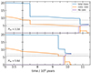 |
Fig. 2. Evolution of the total mass, the convective core mass, and the helium core of the donor model with an initial mass of 20 M⊙ with a companion of initially 14 M⊙ and an initial orbital period of 100.35 d = 2.2 d (top panels) and 100.75 d = 5.6 d (bottom panels). We indicate the mass of the convective core at the onset of mass transfer, just after the fast Case A, and at central hydrogen depletion by grey lines. |
Since the remaining core hydrogen-burning time is larger for the donor in the closer system 3.3 but only (0.4 ⋅ 106 years for the wide system), the mass of the donor’s convective core decreases even more. During the slow Case A phase, the donor transfers mass on a nuclear timescale, wherefore the donor in the close system loses more mass. In the example in Fig. 2, the donor mass at central hydrogen depletion is 9.6 M⊙ for the close and 10.3 M⊙ for the wide system. This causes the mass of the convective core to become even smaller, which forms the second reason for the period dependency. At central hydrogen depletion, the convective cores has shrunken by 1.4 M⊙ since end of fast Case A for the close system and by only 0.2 M⊙ for the wide system. Over the whole model set, this effect can shrink the convective core up to 5 M⊙ for the closest and heaviest systems. For light donors, both effect are equally important, since for close and wide systems the difference in mass change of the convective core for the first effect is about 1 M⊙ as it is for the second one, while for heavier donors, the second one dominates. Finally, the mass of the convective core at hydrogen exhaustion determines the mass of the helium core, which then determines the mass of the donor after Case AB mass transfer.
Figure 3 shows in its top and middle panels the duration of Case A mass transfer as a function of initial donor mass and initial orbital period. We find that the duration is larger for initially closer orbits, since donor stars in close orbits fill their Roche lobe earlier and thus more of the core hydrogen-burning time remains for the donor in its mass-reduced state. Furthermore, the duration of Case A mass transfer increases weakly with increasing initial mass for initial orbital periods above about 100.5 − 0.6 d and decreases for lower initial periods. This means a stronger decrease in duration of mass transfer with initial orbital period for smaller initial donor masses. For our lowest masses (10 M⊙) with the closest orbits, we find durations for Case A mass transfer of about 107 years. Interestingly, for both metallicities the Case A duration is about 106 years around initial orbital periods around 100.5 − 0.6 d, independently of initial donor mass. From the middle plots one can see that the differences in Case A duration between the two metallicities are small and mainly arise from the initial masses and periods where Case A mass transfer is stable. In particular, the upper left corner of the middle panel of Fig. 3 contains models for the LMC grid, but not for the SMC grid. It also shows through the interquartile range that the impact of the initial mass ratio is very small.
 |
Fig. 3. Duration of Case A mass transfer (ΔtA) in logarithmic years as functions of initial orbital period Pini with the initial donor mass Mini colour-coded (top) and as functions of the initial donor mass, where models with the same initial orbital period are indicated with the same colour (middle). The bottom panels show the ratio of the Case A donor core hydrogen-burning lifetime t′MS to the core hydrogen-burning lifetime tMS of a single star of the same initial mass, as a function of the initial orbital period and in the top plots we indicted in black its interquartile range. Each cross represents the median value of ΔtA across different initial mass ratios. In the top plot we indicted in black the first and third quartile. Grey lines indicate our best fit to the data. The panels on the left show LMC models and on the right is SMC. |
In the bottom plot of Fig. 3, we show the ratio of the core hydrogen-burning lifetime of the Case A donor t′MS in units of the core hydrogen-burning lifetime of a single star of the same initial mass tMS. We find that in this representation a strong non-linear correlation to the initial orbital period. The lifetime increases for smaller initial orbital period. This is not unexpected as systems with lower initial orbital period undergo RLO earlier, have thus a larger hydrogen fraction in the core after the fast part of the mass transfer and are less massive and therefore keep core hydrogen-burning for a longer time. We find increases in lifetime of up to 30% for the closest systems. For larger initial orbital periods, the lifetime increase becomes zero as the upper orbital period for Case A mass transfer is reached. For the 10 M⊙-models this happens around an initial period of 100.6 d and for the 40 M⊙-models around 101.4 d (LMC) and 101.2 d (SMC), respectively. The bottom panels show that for the same initial orbital period, the lifetime increase is larger for the larger metallicity.
We find that if we would normalise the data so that we would show the lifetime increase as a function between minimum and maximum of period where Case A mass transfer occurs, they would not lie as neatly on one curve as shown here. Using the orbital period as the independent quantity for Figs. 1 and 3 may seem to be an arbitrary choice, but we find that only with that the data fall onto one single curve. Using the relative age of the donor at beginning of the mass transfer compared to the age of central hydrogen exhaustion of a single star of same initial mass or the central hydrogen content at beginning of the mass transfer as the independent quantity does not yield such unique curves. For practical application, we provide these data with fits in Appendix A.
3.2. Analytic fits
Before we provide fits for the donor mass after Case AB mass transfer and the duration of Case A mass transfer, we give mass-dependent boundaries of initial periods, in which Case A occurs and within which our fits are valid. We find that the lower period limit Pmin for a Case A mass transfer that leads to donor stripping is well described by a parabola

with (a, b, c) = (0.240 ± 0.001, 0.270 ± 0.134, 1.04 ± 0.13) for the LMC and (a, b, c) = (0.114 ± 0.012, 1.72 ± 0.27, 1.37 ± 0.02) for the SMC. On the other hand, the upper period limit for Case A mass transfer Pmax, which is also the boundary towards Case B, is also well described by a parabola

with (a, b, c) = (0.619 ± 0.022, 1.87 ± 0.21, 0.957 ± 0.039) for the LMC and (a, b, c) = (0.535 ± 0.019, 1.31 ± 0.13, 0.897 ± 0.040) for the SMC.
We find third-order polynomials f well fitting to describe the dependency of the donor mass MAB after Case AB mass transfer and its duration ΔtA on the initial donor mass Mini and the initial orbital period Pini. We define m = log Mini/M⊙ and p = Pini/d. With that the polynomials can be written as


The coefficients aij of the fit are given in Table 1 for both metallicities. The root-mean-square relative deviation between model data and fit is in all cases smaller than 3% and the maximum relative deviation reaches about 15% for the worst outlier. We conclude that our fit describes the data well. We indicate the fits in Figs. 1 and 3 (top and middle) with grey lines for selected values of the colour coordinate, which confirms that they match well.
Next, we consider the donor mass after Case AB (MAB) in units of the donor mass after Case B (MB). We find a power law of the form

well fitting. We find (a, b) = (0.841 ± 0.007, −1.253 ± 0.007) for the LMC and (a, b) = (0.657 ± 0.008, −1.487 ± 0.016) for the SMC. The root-mean-square relative deviation between data and fit are 3% and 4% for LMC and SMC, respectively. The maximum relative deviation has relative high values of 15% and 24%. They can be explained with the neglection of mass dependence and the wavy structure in the period dependence (consider e.g. the purple sequence in Fig. 1, bottom). For the SMC data the deviation is so strong as they do not fall so well on a single curve due to the jump between post-Case B mass and highest post-Case AB mass. The fit is shown in Fig. 1 (bottom) in grey.
Finally, we give a fit for the relative increase in core hydrogen-burning lifetime t′MS/tMS again in form of a power law

We find (a, b) = (1.003 ± 0.010, −2.779 ± 0.011) for the LMC and (a, b) = (0.577 ± 0.005, −2.741 ± 0.015) for the SMC best fitting. The root-mean-square relative deviation between data and fit are 0.6% and 0.7% and the maximum relative deviation has values of 5% and 7% for LMC and SMC, respectively. The latter is impacted by the three outliers around Pini ≈ 100.3 d. A visual inspection of the fit in Fig. 3 (bottom, grey line) shows that it does not trace the mass dependence perfectly, meaning that donors with lower initial mass reach unity at lower orbital periods, but such small deviations can safely be disregarded.
The fits for the post-Case AB mass and the lifetime increase are independent of initial donor mass. This suggests that our results may be applicable outside of the considered donor mass range. To test this, we compared our fits to additional detailed models. For the LMC we used models from the extensions of the LMC grid by Pauli et al. (2022), and for the SMC models of our grid outside of the adopted mass range. We show in Table 2 the parameters of the models and compare the outcomes of Case A. We find that the typical deviation between fit and detailed model is less then 10%. Only the lifetime of the 5 M⊙ SMC model and the post-Case AB mass of the 70 M⊙ LMC model deviate more than this. The typical deviation is comparable with the deviations within the analysed models in Sect. 3.1 and thus we conclude that our fits are also applicable outside of their original mass range, at least as long the models have similar structure (i.e. a convective core and a radiative envelope).
Test of our fits against models outside the used mass range (10–40 M⊙).
4. Discussion
4.1. Impact of the initial mass ratio and the accretion efficiency
We have seen in Sect. 3.1 that the post-Case AB mass and the duration of Case A mass transfer are nearly independent of the initial mass ratio (Fig. 1 top panels and Fig. 3 middle panels). This result is further reinforced by the small deviation between data and fits in Sect. 3.2, since the fits do not consider the initial mass ratio and are still very good. We can explain the insensibility of our results to the initial mass ratio by considering each of the three phases of the RLO individually. The onset of interaction at a fixed orbital period happens more or less at the same donor radius, and thus donor age, nearly independent of mass ratio (about a factor of 2 in orbital period over the relevant regime, Eggleton 1983; Marchant & Bodensteiner 2023). The end of the first fast phase of mass transfer is determined by the interplay between the radius evolution of the donor star and the evolution of its Roche radius. The former is a question of stellar physics and the latter mainly depends on the orbital period and is again only a weak function of mass ratio. This is in opposition to Giannone et al. (1968), who predicted larger mass loss from the donor for smaller initial mass ratios (their Fig. 6 in particular). The slow Case A phase is determined by the nuclear evolution of the donor star, on which the accretor star has no impact. Finally, in Case AB mass transfer, which is very similar to Case B, the donor loses mass until its helium core ignites, on which the companion has also no impact. All this is in agreement with Figs. F.3–F.5 of Sen et al. (2022).
It may appear that our model grid could have the shortcoming that we may lose generality by assuming a certain mass transfer evolution during RLO. As the secondary star accretes matter until it reaches critical rotation, tidal forces cause a wide range of mass-transfer efficiencies (Sen et al. 2022, Fig. F.2). The mass-transfer efficiency controls the orbital evolution of the binary through the scheme of isotropic re-emission (Soberman et al. 1997) and thus the size of the donor’s Roche lobe. Thus one wonder whether our results are only valid for these assumptions. It turns out, however, that the accretion efficiency only has a limited effect on the outcome of Case A mass transfer. Consider the 40 M⊙-models of the LMC grid. They show a clear structure in accretion efficiency (Sen et al. 2022, Fig. F.2). When we consider an initial period of 100.6 d, we find for an initial mass ratio of 0.9 an overall accretion efficiency of about 80%, and for an initial mass ratio of 0.55 an accretion efficiency of 30%. Yet in both cases the donor mass after the mass transfer about 18 M⊙ (18.6 M⊙ for the first and 17.5 M⊙ for the latter), which is a strong indication that the accretion efficiency is a subdominant factor. In fact, it turns out that in Fig. 1 (top) the slightly larger interquartile range due to different initial mass ratios in the mid-period regime is caused by the transition from high to low accretion efficiency. (Compare the periods with a larger interquartile range to Fig. F.2 of Sen et al. 2022.) This should also cause the light wiggle in the model data in, for example, Fig. 1 around a period of about 100.5 d. Thus we can quantify the impact of varying accretion efficiency and argue that its effect is small for the whole of both model grids.
4.2. Metallicity dependence
In Sect. 1, we have found that the exponent b of the power law describing the ratio of post-Case A mass to post-Case B mass is smaller for the smaller metallicity. This means that this ratio increases slower with initial orbital periods for the smaller metallicity. However, the smaller offset a in the power law causes the curve of the smaller metallicity to lie on top of the other in the considered period range. Therefore, we conclude that the donor mass after Case A compared with the mass after Case B is larger for smaller metallicities, given the same initial orbital period, and thus models with Galactic metallicity might be even lighter after Case A mass transfer. This can be qualitatively understood by the fact that donor radii at zero-age main-sequence are larger and at higher metallicities and fill their Roche lobe earlier during core hydrogen-burning. Thus they deviate stronger from Case B evolution.
For the increase in the core hydrogen-burning lifetime, we find for both metallicities about same exponent in the power-law fit, namely about −2.8, and that the offset a is larger for the larger metallicity. Therefore, the lifetime increase for the same initial orbital period is larger for the larger metallicity. This fits with the smaller post-Case AB mass for the larger metallicity. Again, we can extrapolate to Galactic metallicity and expect an even stronger lifetime increase.
4.3. Other work
The models we analysed in this work were already compared to observations. Sen et al. (2022) analyse LMC and Milky-Way Algol binaries, which are believed to be a product of Case A mass transfer, with the LMC grid and find a good agreement. Sen et al. (2023) use an extension of the LMC grid by Pauli et al. (2022) to explain so-called revered Algols in the Tarantula Nebula. Wang et al. (2020, 2022) and Wang et al. (2023) find a good agreement of their SMC models with the morphology of Hertzsprung–Russell diagrams, in which systems in slow Case A mass transfer contribute to an extended main-sequence turnoff and blue stragglers.
To calculate the outcome of Case AB mass transfer, several schemes have been adopted in the literature. The BSE-code (Hurley et al. 2002) and its derivatives binary_c (Izzard et al. 2004, 2006, 2009; Schneider et al. 2015) and COMPAS (Stevenson et al. 2017; Riley et al. 2022) determine the post-Case AB donor mass by removing the minimal mass necessary to keep the donor within its Roche-lobe. This process seems to be based on single star models, which neglects the more complex structure (in particular the large helium enriched layer) of a model undergoing Case A mass transfer. Romero-Shaw et al. (2023) propose a simple approximation for the post-Case AB donor mass by multiplying the post-Case B donor mass by the relative age of the donor at the beginning of mass transfer. We show in Fig. A.1 that their method can lead to mismatches of up to 60%. Giannone et al. (1968) follows a more sophisticated approached using generalised main-sequences (stationary models with a particular total mass, central helium abundance and core mass). However, their Fig. 6 shows a clear dependency of the donor mass after fast Case A on the initial mass ratio, which is in contradiction with our results from detailed models. The COMBINE-code of Kruckow et al. (2018) uses the same approach as for Case B to evaluate Case A. They assume that the donor is reduced to its helium core mass. We show in this work that this assumption can be inaccurate to varying degrees, as for core hydrogen-burning models, no helium core can be defined and therefore rely on the helium mass in the convective core. For the duration of Case A they use the thermal timescale, which strongly underestimates its real duration.
5. Conclusions and outlook
In this study we analyse large grids of detailed massive binary evolution models to provide simple recipes for the donor mass after Case AB mass transfer and for the duration of Case A mass transfer. We find that these two quantities are nearly independent of the initial mass ratio of the binary. For the post-Case AB donor mass relative to the post-Case B donor mass, and for the ratio of core hydrogen-burning lifetime compared to that of a single star, we find that power laws (Eqs. (4) and (5)) describe the models well. The main-sequence lifetime of Case A donors exceed that of single stars or Case B donors of the same initial mass by up to 30%. This extension depends on the initial orbital period, but is insensitive to the initial donor mass (Fig. 3, bottom). The donor mass after Case AB can be up to 50% smaller than after a corresponding Case B mass transfer (Fig. 1, bottom). We predict lighter donors after mass transfer and a larger lifetime increase at higher metallicities for given initial orbital periods. We find that our results are independent of the employed mass-transfer efficiency, and find evidence that our results are also valid outside the considered mass range.
The significance of these corrective effect of our new method will be strongly dependent on the specific considered binary population. It will naturally be pronounced for a predicted Algol population, as these objects are undergoing slow Case A mass transfer, which is usually neglected in rapid binary evolution codes. While the overall supernova rate in the nearby Universe is perhaps not significantly affected, the occurrence of these events will be delayed by up to 30% due to the longer core hydrogen-burning lifetime and a longer lifetime of the lighter stripped donor.
The predicted lower donor masses may have an even stronger effect, in particular for initial orbital period distributions that are skewed towards short initial orbital periods. As favoured by the initial mass function, of all supernova progenitors our mass correction will strongly affect that part of the parameter space where most neutron stars are born. Even donor stars with initial masses as high as 16 M⊙ may form white dwarfs (Wellstein et al. 2001). In essence, the number of electron capture supernovae will be reduced. The same applies to black holes, but the vicariously generated neutron stars will not compensate the loss to white dwarfs. Consequently, the number of high mass X-ray binaries is expected to decrease, but only for supergiant X-ray binaries, which reside in close orbits, in contrast to Be/X-ray binaries, which tend to be the outcome of Case B evolution. The corrected mass of the supernova progenitor might affect the predicted neutron star birth kick, which may change the fate of the binary. The impact on the predictions for gravitational wave sources is non-trivial, but the reduced donor masses could lead to less stellar remnant mergers.
While the qualitative effects of Case A mass transfer are described in the literature, this work quantifies them such that they can be implemented into rapid binary population synthesis codes. They can be used to update the predictions of gravitational-wave event rates for different classes of stellar remnants, and they could also be important for the predicted number of double white dwarf binaries in the Milky Way that LISA can detect. In a forthcoming paper we will use our recipe in a rapid binary population synthesis of the population of massive stars after mass transfer in the SMC.
Acknowledgments
PM acknowledges support from the FWO senior postdoctoral fellowship No. 12ZY523N. KS was funded by the National Science Center (NCN), Poland under grant number OPUS 2021/41/B/ST9/00757.
References
- Banyard, G., Sana, H., Mahy, L., et al. 2022, A&A, 658, A69 [NASA ADS] [CrossRef] [EDP Sciences] [Google Scholar]
- Brott, I., de Mink, S. E., Cantiello, M., et al. 2011, A&A, 530, A115 [NASA ADS] [CrossRef] [EDP Sciences] [Google Scholar]
- Byrne, C. M., Stanway, E. R., Eldridge, J. J., McSwiney, L., & Townsend, O. T. 2022, MNRAS, 512, 5329 [NASA ADS] [CrossRef] [Google Scholar]
- Cantiello, M., & Langer, N. 2010, A&A, 521, A9 [NASA ADS] [CrossRef] [EDP Sciences] [Google Scholar]
- Chaboyer, B., & Zahn, J. P. 1992, A&A, 253, 173 [NASA ADS] [Google Scholar]
- de Mink, S. E., Pols, O. R., & Hilditch, R. W. 2007, A&A, 467, 1181 [NASA ADS] [CrossRef] [EDP Sciences] [Google Scholar]
- de Mink, S. E., Langer, N., Izzard, R. G., Sana, H., & de Koter, A. 2013, ApJ, 764, 166 [Google Scholar]
- de Mink, S. E., Sana, H., Langer, N., Izzard, R. G., & Schneider, F. R. N. 2014, ApJ, 782, 7 [Google Scholar]
- Detmers, R. G., Langer, N., Podsiadlowski, P., & Izzard, R. G. 2008, A&A, 484, 831 [NASA ADS] [CrossRef] [EDP Sciences] [Google Scholar]
- Eggleton, P. P. 1983, ApJ, 268, 368 [Google Scholar]
- Eldridge, J. J., Izzard, R. G., & Tout, C. A. 2008, MNRAS, 384, 1109 [Google Scholar]
- Eldridge, J. J., Stanway, E. R., Xiao, L., et al. 2017, PASA, 34, e058 [Google Scholar]
- Fragos, T., Andrews, J. J., Bavera, S. S., et al. 2023, ApJS, 264, 45 [NASA ADS] [CrossRef] [Google Scholar]
- Giannone, P., Kohl, K., & Weigert, A. 1968, Z. Astrophys., 68, 107 [NASA ADS] [Google Scholar]
- Han, Z.-W., Ge, H.-W., Chen, X.-F., & Chen, H.-L. 2020, Res. Astron. Astrophys., 20, 161 [CrossRef] [Google Scholar]
- Heger, A., Langer, N., & Woosley, S. E. 2000, ApJ, 528, 368 [NASA ADS] [CrossRef] [Google Scholar]
- Heger, A., Woosley, S. E., & Spruit, H. C. 2005, ApJ, 626, 350 [Google Scholar]
- Hurley, J. R., Pols, O. R., & Tout, C. A. 2000, MNRAS, 315, 543 [Google Scholar]
- Hurley, J. R., Tout, C. A., & Pols, O. R. 2002, MNRAS, 329, 897 [Google Scholar]
- Iglesias, C. A., & Rogers, F. J. 1996, ApJ, 464, 943 [NASA ADS] [CrossRef] [Google Scholar]
- Izzard, R. G., Tout, C. A., Karakas, A. I., & Pols, O. R. 2004, MNRAS, 350, 407 [CrossRef] [Google Scholar]
- Izzard, R. G., Dray, L. M., Karakas, A. I., Lugaro, M., & Tout, C. A. 2006, A&A, 460, 565 [NASA ADS] [CrossRef] [EDP Sciences] [Google Scholar]
- Izzard, R. G., Glebbeek, E., Stancliffe, R. J., & Pols, O. R. 2009, A&A, 508, 1359 [NASA ADS] [CrossRef] [EDP Sciences] [Google Scholar]
- Kruckow, M. U., Tauris, T. M., Langer, N., Kramer, M., & Izzard, R. G. 2018, MNRAS, 481, 1908 [CrossRef] [Google Scholar]
- Langer, N. 1991, A&A, 252, 669 [NASA ADS] [Google Scholar]
- Langer, N. 1998, A&A, 329, 551 [NASA ADS] [Google Scholar]
- Langer, N. 2012, ARA&A, 50, 107 [CrossRef] [Google Scholar]
- Langer, N., Fricke, K. J., & Sugimoto, D. 1983, A&A, 126, 207 [NASA ADS] [Google Scholar]
- Langer, N., Schürmann, C., Stoll, K., et al. 2020, A&A, 638, A39 [NASA ADS] [CrossRef] [EDP Sciences] [Google Scholar]
- Laplace, E., Götberg, Y., de Mink, S. E., Justham, S., & Farmer, R. 2020, A&A, 637, A6 [NASA ADS] [CrossRef] [EDP Sciences] [Google Scholar]
- Laplace, E., Justham, S., Renzo, M., et al. 2021, A&A, 656, A58 [NASA ADS] [CrossRef] [EDP Sciences] [Google Scholar]
- Lipunov, V. M., Postnov, K. A., & Prokhorov, M. E. 1996, A&A, 310, 489 [NASA ADS] [Google Scholar]
- Lubow, S. H., & Shu, F. H. 1975, ApJ, 198, 383 [NASA ADS] [CrossRef] [Google Scholar]
- Marchant, P. 2017, Ph.D. Thesis, Rheinische Friedrich Wilhelms University of Bonn, Germany [Google Scholar]
- Marchant, P., & Bodensteiner, J. 2023, arXiv e-prints [arXiv:2311.01865] [Google Scholar]
- Menon, A., Langer, N., de Mink, S. E., et al. 2021, MNRAS, 507, 5013 [NASA ADS] [CrossRef] [Google Scholar]
- Moe, M., & Di Stefano, R. 2017, ApJS, 230, 15 [Google Scholar]
- Nelson, C. A., & Eggleton, P. P. 2001, ApJ, 552, 664 [NASA ADS] [CrossRef] [Google Scholar]
- Pauli, D., Langer, N., Aguilera-Dena, D. R., Wang, C., & Marchant, P. 2022, A&A, 667, A58 [NASA ADS] [CrossRef] [EDP Sciences] [Google Scholar]
- Paxton, B., Bildsten, L., Dotter, A., et al. 2011, ApJS, 192, 3 [Google Scholar]
- Paxton, B., Cantiello, M., Arras, P., et al. 2013, ApJS, 208, 4 [Google Scholar]
- Paxton, B., Marchant, P., Schwab, J., et al. 2015, ApJS, 220, 15 [Google Scholar]
- Petrovic, J., Langer, N., & van der Hucht, K. A. 2005, A&A, 435, 1013 [NASA ADS] [CrossRef] [EDP Sciences] [Google Scholar]
- Podsiadlowski, P., Joss, P. C., & Hsu, J. J. L. 1992, ApJ, 391, 246 [Google Scholar]
- Pols, O. R. 1994, A&A, 290, 119 [Google Scholar]
- Renzo, M., & Götberg, Y. 2021, ApJ, 923, 277 [NASA ADS] [CrossRef] [Google Scholar]
- Renzo, M., Zapartas, E., Justham, S., et al. 2023, ApJ, 942, L32 [NASA ADS] [CrossRef] [Google Scholar]
- Riley, J., Agrawal, P., Barrett, J. W., et al. 2022, ApJS, 258, 34 [NASA ADS] [CrossRef] [Google Scholar]
- Romero-Shaw, I., Hirai, R., Bahramian, A., Willcox, R., & Mandel, I. 2023, MNRAS, 524, 245 [NASA ADS] [CrossRef] [Google Scholar]
- Sana, H., de Mink, S. E., de Koter, A., et al. 2012, Science, 337, 444 [Google Scholar]
- Sana, H., de Koter, A., de Mink, S. E., et al. 2013, A&A, 550, A107 [NASA ADS] [CrossRef] [EDP Sciences] [Google Scholar]
- Schneider, F. R. N., Izzard, R. G., Langer, N., & de Mink, S. E. 2015, ApJ, 805, 20 [Google Scholar]
- Schootemeijer, A., Langer, N., Grin, N. J., & Wang, C. 2019, A&A, 625, A132 [NASA ADS] [CrossRef] [EDP Sciences] [Google Scholar]
- Sen, K., Langer, N., Marchant, P., et al. 2022, A&A, 659, A98 [NASA ADS] [CrossRef] [EDP Sciences] [Google Scholar]
- Sen, K., Langer, N., Pauli, D., et al. 2023, A&A, 672, A198 [NASA ADS] [CrossRef] [EDP Sciences] [Google Scholar]
- Shao, Y., & Li, X.-D. 2021, ApJ, 908, 67 [NASA ADS] [CrossRef] [Google Scholar]
- Soberman, G. E., Phinney, E. S., & van den Heuvel, E. P. J. 1997, A&A, 327, 620 [NASA ADS] [Google Scholar]
- Spruit, H. C. 2002, A&A, 381, 923 [CrossRef] [EDP Sciences] [Google Scholar]
- Stanway, E. R., & Eldridge, J. J. 2018, MNRAS, 479, 75 [NASA ADS] [CrossRef] [Google Scholar]
- Stevenson, S., Vigna-Gómez, A., Mandel, I., et al. 2017, Nat. Commun., 8, 14906 [Google Scholar]
- Ulrich, R. K., & Burger, H. L. 1976, ApJ, 206, 509 [NASA ADS] [CrossRef] [Google Scholar]
- Vanbeveren, D., & De Loore, C. 1994, A&A, 290, 129 [NASA ADS] [Google Scholar]
- Vanbeveren, D., van Bever, J., & De Donder, E. 1997, A&A, 317, 487 [NASA ADS] [Google Scholar]
- Vanbeveren, D., De Donder, E., Van Bever, J., Van Rensbergen, W., & De Loore, C. 1998, New Astron., 3, 443 [CrossRef] [Google Scholar]
- Vigna-Gómez, A., Neijssel, C. J., Stevenson, S., et al. 2018, MNRAS, 481, 4009 [Google Scholar]
- Wang, C., Langer, N., Schootemeijer, A., et al. 2020, ApJ, 888, L12 [NASA ADS] [CrossRef] [Google Scholar]
- Wang, C., Langer, N., Schootemeijer, A., et al. 2022, Nat. Astron., 6, 480 [NASA ADS] [CrossRef] [Google Scholar]
- Wang, C., Hastings, B., Schootemeijer, A., et al. 2023, A&A, 670, A43 [NASA ADS] [CrossRef] [EDP Sciences] [Google Scholar]
- Wellstein, S., Langer, N., & Braun, H. 2001, A&A, 369, 939 [NASA ADS] [CrossRef] [EDP Sciences] [Google Scholar]
Appendix A: Fits as a function of main-sequence lifetime
For the application of our results, it may be more practical to use the ratio of the time tRLO when the RLO begins to the main-sequence lifetime tMS of the donor as the independent quantity instead of the initial orbital period. We show this in Fig. A.1. The ratio of the post-Case AB mass to the post-Case B mass increases and the core hydrogen-burning lifetime decreases with tRLO/tMS. In this representation the two quantities become mass-dependent again. For the mass after Case AB, we find a rational function of the form

well fitting. We find (a, b, c, d) = (2.76 ± 0.03, −3.75 ± 0.05, −1.60 ± 0.04, 3.47 ± 0.05) for the LMC and (a, b, c, d) = (2.03 ± 0.07, −2.50 ± 0.10, −0.86 ± 0.08, 2.21 ± 0.11) for the SMC. The root-mean-square relative deviations are 2% and 4%, and the maximum relative deviations are 12% and 21%, respectively.
For the increase in core hydrogen-burning lifetime, we find a power law of the form

well fitting. We find (a, b, c) = (116.8 ± 1.7, 1.618 ± 0.004, 1.465 ± 0.003) for the LMC and (a, b, c) = (80.5 ± 4.7, 1.438 ± 0.016, 1.649 ± 0.012) for the SMC. The root-mean-square relative deviations are 0.3% and 0.9%, and the maximum relative deviations are 4% and 6%, respectively.
 |
Fig. A.1. Same as Fig. 1 (top, also top here) and 3 (top, here bottom), but as a function of the fraction in the donor core hydrogen-burning lifetime when the RLO begins. Grey lines indicate our best fit to the data and the dashed black line shows the approach of Romero-Shaw et al. (2023), i.e. MAB = MBtRLO/tMS. The panels on the left show LMC models, and on the right SMC show models. |
All Tables
All Figures
|
Fig. 1. Donor mass immediately after Case AB mass transfer (MAB) in units of the solar mass (top and middle) and in units of the donor mass after Case B mass transfer (MB, bottom), as a function of the initial orbital period Pini, with the initial donor mass Mini colour-coded (top and bottom). The middle panel shows MAB as a function of the initial donor mass, where models with the same initial orbital period are indicated with the same colour. Each cross represents the median of MAB across different initial mass ratios and in the top plots we indicted in black its interquartile range (distance from first to third quartile of the mass ratio distribution). In the middle plots the black lines show the mass of the convective cores of single stars at the beginning (MZAMSconv.core) and the end (MTAMSconv.core) of core hydrogen-burning, as well as the mass after Case B mass transfer, as a function of the initial stellar mass. Grey lines indicate our best fit to the data. The panels on the left show LMC models, and on the right SMC show models. |
| In the text | |
|
Fig. 2. Evolution of the total mass, the convective core mass, and the helium core of the donor model with an initial mass of 20 M⊙ with a companion of initially 14 M⊙ and an initial orbital period of 100.35 d = 2.2 d (top panels) and 100.75 d = 5.6 d (bottom panels). We indicate the mass of the convective core at the onset of mass transfer, just after the fast Case A, and at central hydrogen depletion by grey lines. |
| In the text | |
|
Fig. 3. Duration of Case A mass transfer (ΔtA) in logarithmic years as functions of initial orbital period Pini with the initial donor mass Mini colour-coded (top) and as functions of the initial donor mass, where models with the same initial orbital period are indicated with the same colour (middle). The bottom panels show the ratio of the Case A donor core hydrogen-burning lifetime t′MS to the core hydrogen-burning lifetime tMS of a single star of the same initial mass, as a function of the initial orbital period and in the top plots we indicted in black its interquartile range. Each cross represents the median value of ΔtA across different initial mass ratios. In the top plot we indicted in black the first and third quartile. Grey lines indicate our best fit to the data. The panels on the left show LMC models and on the right is SMC. |
| In the text | |
|
Fig. A.1. Same as Fig. 1 (top, also top here) and 3 (top, here bottom), but as a function of the fraction in the donor core hydrogen-burning lifetime when the RLO begins. Grey lines indicate our best fit to the data and the dashed black line shows the approach of Romero-Shaw et al. (2023), i.e. MAB = MBtRLO/tMS. The panels on the left show LMC models, and on the right SMC show models. |
| In the text | |
Current usage metrics show cumulative count of Article Views (full-text article views including HTML views, PDF and ePub downloads, according to the available data) and Abstracts Views on Vision4Press platform.
Data correspond to usage on the plateform after 2015. The current usage metrics is available 48-96 hours after online publication and is updated daily on week days.
Initial download of the metrics may take a while.