| Issue |
A&A
Volume 690, October 2024
|
|
|---|---|---|
| Article Number | L15 | |
| Number of page(s) | 6 | |
| Section | Letters to the Editor | |
| DOI | https://doi.org/10.1051/0004-6361/202452276 | |
| Published online | 21 October 2024 | |
Letter to the Editor
Spectral characteristics of a rotating solar prominence in multiple wavelengths
1
Centre for mathematical Plasma Astrophysics, KU Leuven, Celestijnenlaan 200B, 3001
Leuven, Belgium
2
Leibniz-Institut für Astrophysik Potsdam (AIP), An der Sternwarte 16, 14482
Potsdam, Germany
3
SUPA School of Physics and Astronomy, University of Glasgow, Glasgow, G12 8QQ
UK
Received:
17
September
2024
Accepted:
3
October
2024
We present synthetic spectra corresponding to a 2.5D magnetohydrodynamic simulation of a rotating prominence in the Ca II 8542 Å, H α, Ca II K, Mg II k, Ly α, and Ly β lines. The prominence rotation resulted from angular momentum conservation within a flux rope where asymmetric heating imposed a net rotation prior to the thermal-instability-driven condensation phase. The spectra were created using a library built on the Lightweaver framework called Promweaver, which provides boundary conditions for incorporating the limb-darkened irradiation of the solar disk on isolated structures such as prominences. Our spectra show distinctive rotational signatures for the Mg II k, Ly α, and Ly β lines, even in the presence of complex, turbulent solar atmospheric conditions. However, these signals are barely detectable for the Ca II 8542 Å, H α, and Ca II K spectral lines. Most notably, we find only a very faint rotational signal in the H α line, thus reigniting the discussion on the existence of sustained rotation in prominences.
Key words: magnetohydrodynamics (MHD) / radiative transfer / Sun: atmosphere / Sun: corona / Sun: filaments / prominences
Corresponding author; [email protected]
© The Authors 2024
 Open Access article, published by EDP Sciences, under the terms of the Creative Commons Attribution License (https://creativecommons.org/licenses/by/4.0), which permits unrestricted use, distribution, and reproduction in any medium, provided the original work is properly cited.
This article is published in open access under the Subscribe to Open model. Subscribe to A&A to support open access publication.
1. Introduction
Prominences are cold and dense coronal structures that appear in positive contrast against their background when protruding above the solar limb, and in a negative contrast when seen on-disk (in this case, they are termed “filaments”). In both cases, complex magnetic fields such as flux ropes (FRs) and sheared arcades are responsible for the suspension of these structures (Mackay et al. 2010; Terradas et al. 2016). Due to their suspension within the solar corona, prominences are commonly considered to be subject to low plasma-β dynamics, which means that the plasma motions are dominated by magnetic tension and magnetic pressure dynamics (e.g., Jenkins & Keppens 2021; Brughmans et al. 2022; Jerčić et al. 2024). Such bounding to the local magnetic field strongly indicates that the highly dynamic nature of prominence plasma thus maps directly to the underlying field topology since the magnetic field acts to guide the trajectory of the associated plasma. A commonly studied example of such field-aligned dynamics is rotation, which was first described by Secchi (1875) as “spiral structures,” and later by Young (1896) as “whirling waterspouts,” but is primarily attributed to Pettit (1925) under the nomenclature “prominence tornadoes.”
Since then, these events have been reported more frequently. Numerous instances have been studied in the feet of prominences (Su et al. 2012, 2014; Orozco Suárez et al. 2012; Yan et al. 2013, 2014; Wedemeyer et al. 2013; Wedemeyer & Steiner 2014) as well as within coronal cavities (Öhman 1969; Liggett & Zirin 1984; Schmit et al. 2009; Wang & Stenborg 2010a; Li et al. 2012; Mishra et al. 2020), with estimated rotational velocities ranging from 5 to 75 km s−1. The events observed within cavities are thought to be plasma moving along a helical FR, which appears as rotational motion when observed along the axis of the helix (Li et al. 2012; Panasenco et al. 2014). Over time, these flows along a helical FR may lead to plasma drainage down to one of the FR footpoints (Wang & Stenborg 2010a; Wang et al. 2017). Unlike the more unequivocal rotational motions observed in erupting FRs as they unwind, the sustained rotations (> 1 h) of prominences have recently been called into doubt by Levens (2018) and Gunár et al. (2023), who suggest that such motions can also be explained as oscillations, counter-streaming flows, and non-rotational 3D movements projected in such a way that they resemble helical motions. Over the last decade, 2D and 3D magnetohydrodynamic simulations of the formation and evolution of solar prominences have improved dramatically to where current simulations (e.g., Jenkins & Keppens 2021, 2022; Donné & Keppens 2024) exceed the resolution of most observations and are comparable to those of the new Daniel K. Inouye Solar Telescope (Rast et al. 2021).
Recently, Liakh & Keppens (2023) presented the self-consistent emergence of sustained rotation in plasma motions within a cavity, using a 2.5D magnetohydrodynamic simulation of the levitation-condensation scenario of the prominence formation in a nonadiabatic, gravitationally stratified coronal volume, accounting for the effects of turbulent heating at the footpoints. The FR-embedded prominence forms due to thermal instability as lower-lying coronal matter gets levitated during the FR formation, and the contracting condensation inevitably starts rotating.
Simulated Atmospheric Imaging Assembly (AIA; Lemen et al. 2012) proxies (e.g., Xia et al. 2014; Van Doorsselaere et al. 2016; Gibson et al. 2016) and synthetic spectra act as a link between simulations and observations. While the former have been widely employed over the last decade, use of the latter has only recently come into fashion for more detailed prominence models. The reason is twofold: (i) the recent advent of self-consistent prominence formation and evolution models and (ii) the relative difficulty of synthesizing spectral lines that form outside of local thermodynamic equilibrium conditions (e.g., Jenkins et al. 2023, 2024). Only recently have full multidimensional nonlocal thermodynamic equilibrium transfer computations on such highly resolved prominence models become a possibility (Osborne & Sannikov 2024).
In this work we used Promweaver1, a library built on the Lightweaver framework (Osborne & Milić 2021), to forward-model the simulation presented in Liakh & Keppens (2023). We present, for the first time, spectral information on how rotating structures such as the one described in this work would appear if observed, and whether or not the rotational signal is clear enough to be distinguished in a turbulent solar atmosphere.
2. Simulations with MPI-AMRVAC
We used the 2.5D numerical simulation presented in Liakh & Keppens (2023). It shows a systematically rotating prominence within the coronal cavity, which is driven in a way similar as that described in Wang & Stenborg (2010b). While this Letter provides a brief overview of the numerical model and its evolution, a comprehensive description is available in Liakh & Keppens (2023).
The numerical experiment was performed using the open source, adaptive-grid, parallelized Adaptive Mesh Refinement Versatile Advection Code2 (MPI-AMRVAC; Porth et al. 2014; Xia et al. 2018; Keppens et al. 2020, 2023). The simulation box has a domain of 48 × 144 Mm (65 × 195″) with adaptive mesh refinement achieving a minimum grid cell size of 31.25 km (0.04″). The initial magnetic field configuration consists of a force-free sheared arcade, as described by Jenkins & Keppens (2021). Converging and shearing motions at the bottom boundary (for the Vx and Vz velocities) were implemented to form the FR according to van Ballegooijen & Martens (1989).
To simulate turbulent heating from the lower solar atmosphere, randomized heating was included at the bottom of the numerical domain, as in Zhou et al. (2020), Li et al. (2022a), and Jerčić et al. (2024). This heating significantly influences the FR formation, introducing asymmetry into temperature and density distributions with respect to the polarity inversion line. This leads to a coherent flow along magnetic loops, which evolves into a rotational pattern as a twisted FR forms. The plasma near the FR center continues rotating for over an hour, initially reaching speeds of over 60 km s−1. Prominence plasma located farther from the FR center forms at the apex, drains down, and oscillates around the bottom of magnetic dips with a velocity amplitude of approximately 30 km s−1. This is demonstrated by means of synthesized AIA images of the 304, 211, 193, and 171 Å channels (Fig. 4 of Liakh & Keppens 2023) that show the simultaneous rotation of both coronal plasma and condensations as well as the formation of the coronal cavity and dimming region in the overlying loops.
The simulation ran for 1000 time steps with a ∼8.59 s cadence, for a total of 142 minutes. In Fig. 1 the density distribution at the start, middle, and end of the simulation is shown, and the rotation is illustrated in movie 1. The condensation tail forms later on and remains oscillating until the final stage of the numerical experiment. The MPI-AMRVAC data solved on an adaptive mesh refinement grid were converted into uniformly spaced NetCDF (Rew & Davis 1990) files using the yt-project (Turk et al. 2011).
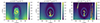 |
Fig. 1. Density distribution in the central part of the numerical domain at 42, 80, and 142 minutes, showing the different stages of evolution of the prominence as well as the longevity of the rotational motion. An animated version of this figure is available online (see movie 1). |
3. Spectral synthesis with Promweaver
Promweaver is an extension to the Lightweaver framework designed for modeling isolated structures within the solar atmosphere. As of v0.3.0 (Osborne et al. 2024), it provides simplified classes for the boundary conditions as described in Jenkins et al. (2023) and for employing these with stratified atmospheres (such as columns from MPI-AMRVAC) while optionally conserving charge and pressure (Jerčić et al. 2024). The boundary conditions employed in Promweaver sample the limb-darkened radiation emerging from the solar disk arriving at the prominence and can self-consistently account for Doppler shifts relative to the disk (see also Peat et al. 2024). We adopted a semi-empirical FAL-C (Fontenla et al. 1993) as a reference quiet-Sun model. The limb-darkened radiation across the spectral range of interest was tabulated from this model via a plane-parallel treatment, which serves as an input for the boundary conditions. This library also contains classes for reproducing the PROM code series of models (e.g., Gouttebroze et al. 1993; Heinzel et al. 1994) for both the isothermal and isobaric cases, as well as those with a prominence corona transition region (as described in Labrosse & Gouttebroze 2004).
The Lightweaver framework (Osborne & Milić 2021) employs the multilevel accelerated lambda iteration approach from Rybicki & Hummer (1992), the iterative procedure for determining partial frequency redistribution from Uitenbroek (2001), and the hybrid partial frequency redistribution approximation for moving atmospheres as described in Leenaarts et al. (2012). We used the standard settings for the formal solver and interpolation techniques. In this work, we modeled and investigated spectral lines of H, Ca II, and Mg II. Partial frequency redistribution was employed for the resonance lines investigated for all of these species, namely Lyman α & β, Ca II K & 8542 Å, and Mg II k. Similarly to Jenkins et al. (2023), we find that the signal produced by the other two lines of the Ca II IR triplet, as well as Ca II H and Mg II h, are nearly identical to their counterparts, and we thus left them out of our analysis.
4. Results and discussion
In this study we considered two axis-aligned projections, a top-down view that we dub the “filament view” and a sideways “prominence view.” This is illustrated in the second and third columns of Fig. 2, where vertical and horizontal rays can be seen for the filament and prominence view, respectively. The first column shows the synthetic H α profiles obtained from the synthesizing of these rays together with the appropriate FAL-C boundary conditions. The second column shows the density map in the same units as Fig. 1. The third column shows the line-of-sight velocity (e.g., along the integration direction). Animated versions of the two figures are available online (see movie 2 and movie 3).
 |
Fig. 2. Example synthesized spectra along three rays at t = 85 min. We show a ray representing the background (in black), rotating condensation (in red), and an oscillating tail (in blue). The top row shows the spectra resulting from filament synthesis, with the three rays marked on the line-of-sight velocity and density map. Here the black line overlaps with the red line everywhere except at the red wing. The bottom row shows the same but for prominence synthesis, with the black line being close to zero across the spectrum. An animated version of both views is available online (see movie 2 and movie 3). |
The black line in both views represents a “quiet” reference profile, which is traced through a part of the simulation where the prominence density is too low to affect the underlying FAL-C atmosphere. The red line crosses a high-density rotating kernel that manifests itself in both views as a redshifted signal of approximately 60 km s−1. The blue line crosses the high-density oscillating condensation tail below the rotating part of the prominence. The much lower velocities of this region do not noticeably shift the profile, but the increased column mass results in an opacity broadening of the line as well as a saturation of the line core in the filament view. This is in line with Leenaarts et al. (2012), who show that the H α line opacity is mainly sensitive to mass density under chromospheric conditions. These resulting spectra are also similar to the observations shown in Fig. 6 of Schwartz et al. (2019) and Fig. 2 of Kuckein et al. (2016), demonstrating that this tail is similar to typical prominence plasma.
We repeated the synthesis steps for both views across the entire time series. However, due to the relatively high computational cost of creating these spectra, we opted to sample the data sparsely in both the temporal and spatial directions. Every tenth snapshot was temporally synthesized, resulting in 100 snapshots spanning the full 142-minute duration of the simulation with an 86 s cadence. Spatially, each snapshot was sampled at each 16th column, resulting in 100 columns across the 50 Mm domain for an effective resolution of 0.5 Mm, or 0.68″. This is within an order of magnitude of current-generation ground- and space-based telescopes (e.g., Scharmer et al. 2003; De Pontieu et al. 2014; Li et al. 2022b). On a 2022 MacBook Air, a single snapshot at this sparse resolution takes an average of six hours to complete. We have not exploited the sparsity of the model as large fractions of many columns have temperatures in the megakelvin regime and are not meaningfully involved in the radiative transfer calculation but still consume memory and processing power.
In Figs. 3 and 4 we show a simulated spectral slit across the line of sight of the filament and prominence, respectively, in the Ca II 8542 Å, H α, Ca II K, Mg II k, Ly α, and Ly β lines, ordered from low to high disk formation heights (e.g., de la Cruz Rodríguez et al. 2019, Fig. 1). Both slits correspond to the atmosphere of the same snapshot as shown in Fig. 2 at 85 minutes into the simulation, with each ray in the spectral direction corresponding to one synthesized spectrum. In both cases, we find that only the high-density rotating kernel and condensed oscillating tail affect the underlying spectrum. The evolution of the entire time series can be viewed in movie 4 and movie 5.
 |
Fig. 3. Simulated spectral slit across the filament view at t = 85 min (see the first row of Fig. 2.), showing the Ca II 8542 Å, H α, Ca II K, Mg II k, Ly α, and Ly β lines. An animated version of this figure is available online (movie 4). |
 |
Fig. 4. Same as Fig. 3 but for the prominence view. An animated version of this figure is available online (movie 5). |
4.1. Filament view
In the filament view, hardly any signal can be perceived in Ca II 8542 Å throughout the time series. In H α and Ca II K we are primarily sensitive to the higher-density condensation tail, which manifests itself as an absorption feature in the line core and primarily moves around in the spatial direction, showing very little Doppler shift. The rotating kernel manifests itself faintly as a highly Doppler-shifted (∼60 km s−1) absorption feature that alternates between red- and blueshifts, much like the red line in Fig. 2. The signal of the rotating kernel seems most distinct in Mg II k, where a stronger absorption feature can be seen stretching across the spectral dimension, while in the Lyman lines the signals of the two features overlap significantly.
To our knowledge, there are no studies focusing on the evolution of filament spectra at a single location, and thus a direct comparison with observations is difficult. However, the synthetic spectra have shifts on the same order of magnitude as the erupting filament observed by Madjarska et al. (2022).
4.2. Prominence view
In the prominence view, the signal is scaled to a tenth of the continuum for the top row, a quarter of the emission peak for Mg II k, and to the emission peak in the Lyman lines. Here we find a similar result to that of the filament view, where the rotating feature is best seen in the magnesium and hydrogen resonance lines, while barely being visible in the two lower-forming lines. Likewise, two Doppler patterns are visible: the high-density condensation tail between 15 and 20 Mm and the rotating kernel between 20 and 30 Mm. The former shows what seems to be a broadening but is in fact the “back-and-forth” motion of the tail. The rotating component produces a diagonal component on the slit that exhibits the strongest Doppler shifts when the rotating kernel is in the lower-left or upper-right position, moving primarily in the direction of the line of sight. The rotational signal is once again best seen in the Mg II k line. The signature left by the rotating kernel has a close resemblance to the observations shown in Fig. 8 of Barczynski et al. (2023) and to a lesser degree the spectra shown in Fig. 7 of Barczynski et al. (2021), which more closely resemble the oscillating tail.
4.3. Model dimensionality
An important limitation of this work is the dimensionality of the model used to synthesize these results, as 2.5D simulations of prominence formation and evolution often underestimate the total prominence mass due to the limited plasma reservoir available. In contrast, a 3D model allows for more realistic plasma evaporation driven by randomized heating at the footpoints of the anchored FR. The resulting increase in total prominence mass has significant implications for spectral synthesis, especially for optically thick lines like H α, which are highly sensitive to density variations. Additionally, as discussed in Liakh & Keppens (2023), the 2.5D setup cannot account for certain key physical processes, such as field-aligned pressure gradients, leading to a lack of physical attenuation of motions. Finally, in a 3D FR model, rotational flows will eventually result in plasma drainage at one of the footpoints, a process important for understanding the life cycle and stability of prominences. Future work can build on recent full 3D models of realistic prominences as simulated by Donné & Keppens (2024).
5. Conclusions
Following the procedure laid out in Jenkins et al. (2023), we used Promweaver, a library built on Lightweaver, to create synthetic spectra of the 2.5D MPI-AMRVAC simulation presented in Liakh & Keppens (2023) in a sideways (prominence) and top-down (filament) view. The simulation was sampled sparsely at a resolution of 0.68″ (0.5 Mm) and a cadence of 86 s, spanning 142 minutes, for the 65 × 195″ (48 × 144 Mm) simulation box. The resulting spectra of the Ca II 8542 Å, H α, Ca II K, Mg II k, Ly α, and Ly β lines are shown for one snapshot in Figs. 3 and 4, and the full-time series can be viewed in movie 4 and movie 5.
In both views we find a Doppler signature left by the continuously rotating kernel of up to 60 km s−1. However, in both views the visibility of the effect is negligible in Ca II 8542 Å, and barely detectable in H α and Ca II K. The Mg II k line gives the clearest signal, while the Lyman lines show a blended response between the condensed oscillating tail and the rotating kernel, which may be harder to disentangle for slower rotations.
Our current findings suggest that the nature of rotating prominences makes their rotational component challenging to detect in classically used lines such as H α, although this may improve once a 3D prominence model is created and studied in the same way. However, this could explain why no such effects were found by Levens (2018) and Gunár et al. (2023). For this reason, we suggest that future observational studies focus on the Interface Region Spectrograph (IRIS; De Pontieu et al. 2014), which uses sparse, high signal-to-noise Mg II rasters to hunt for such signals in both filaments and prominences.
Data availability
Movies are available at https://www.aanda.org
Promweaver: https://zenodo.org/records/11358632
Acknowledgments
RK and AP received funding from the European Research Council (ERC) under the European Union Horizon 2020 research and innovation program (grant agreement No. 833251 PROMINENT ERC-ADG 2018) and RK is supported by FWO projects G0B4521N and G0B9923N. CMJO is grateful for the support of a Royal Astronomical Society fellowship. We acknowledge productive discussions with Dr Veronika Jerčić, Dr Malcolm Druett, and thank the anonymous referee for their valuable suggestions during the peer-review process. This research has made use of NASA’s Astrophysics Data System (ADS) bibliographic services. We acknowledge the community efforts devoted to the development of the following open-source packages that were used in this work: numpy (numpy.org), matplotlib (matplotlib.org), and astropy (astropy.org).
References
- Barczynski, K., Schmieder, B., Peat, A. W., et al. 2021, A&A, 653, A94 [NASA ADS] [CrossRef] [EDP Sciences] [Google Scholar]
- Barczynski, K., Schmieder, B., Gelly, B., Peat, A. W., & Labrosse, N. 2023, A&A, 680, A63 [NASA ADS] [CrossRef] [EDP Sciences] [Google Scholar]
- Brughmans, N., Jenkins, J. M., & Keppens, R. 2022, A&A, 668, A47 [NASA ADS] [CrossRef] [EDP Sciences] [Google Scholar]
- de la Cruz Rodríguez, J., Leenaarts, J., Danilovic, S., & Uitenbroek, H. 2019, A&A, 623, 623 [Google Scholar]
- De Pontieu, B., Title, A. M., & Lemen, J. R. 2014, Sol. Phys., 289, 2733 [NASA ADS] [CrossRef] [Google Scholar]
- Donné, D., & Keppens, R. 2024, ApJ, 971, 90 [CrossRef] [Google Scholar]
- Fontenla, J. M., Avrett, E. H., & Loeser, R. 1993, ApJ, 406, 319 [Google Scholar]
- Gibson, S., Kucera, T., White, S., et al. 2016, Front. Astron. Space Sci., 3, 8 [NASA ADS] [CrossRef] [Google Scholar]
- Gouttebroze, P., Heinzel, P., & Vial, J. C. 1993, A&AS, 99, 513 [NASA ADS] [Google Scholar]
- Gunár, S., Labrosse, N., Luna, M., et al. 2023, Space Sci. Rev., 219, 33 [CrossRef] [Google Scholar]
- Heinzel, P., Gouttebroze, P., & Vial, J. C. 1994, A&A, 292, 656 [NASA ADS] [Google Scholar]
- Jenkins, J. M., & Keppens, R. 2021, A&A, 646, A134 [NASA ADS] [CrossRef] [EDP Sciences] [Google Scholar]
- Jenkins, J. M., & Keppens, R. 2022, Nat. Astron., 6, 942 [NASA ADS] [CrossRef] [Google Scholar]
- Jenkins, J. M., Osborne, C. M. J., & Keppens, R. 2023, A&A, 670, A179 [NASA ADS] [CrossRef] [EDP Sciences] [Google Scholar]
- Jenkins, J. M., Osborne, C. M. J., Qiu, Y., Keppens, R., & Li, C. 2024, ApJ, 964, L34 [NASA ADS] [CrossRef] [Google Scholar]
- Jerčić, V., Jenkins, J. M., & Keppens, R. 2024, A&A, 688, A145 [NASA ADS] [CrossRef] [EDP Sciences] [Google Scholar]
- Keppens, R., Teunissen, J., Xia, C., & Porth, O. 2020, arXiv e-prints [arXiv:2004.03275] [Google Scholar]
- Keppens, R., Popescu Braileanu, B., Zhou, Y., et al. 2023, A&A, 673, A66 [NASA ADS] [CrossRef] [EDP Sciences] [Google Scholar]
- Kuckein, C., Verma, M., & Denker, C. 2016, A&A, 589, A84 [NASA ADS] [CrossRef] [EDP Sciences] [Google Scholar]
- Labrosse, N., & Gouttebroze, P. 2004, ApJ, 617, 614 [NASA ADS] [CrossRef] [Google Scholar]
- Leenaarts, J., Pereira, T., & Uitenbroek, H. 2012, A&A, 543, A109 [NASA ADS] [CrossRef] [EDP Sciences] [Google Scholar]
- Lemen, J. R., Title, A. M., Akin, D. J., et al. 2012, Sol. Phys., 275, 17 [Google Scholar]
- Levens, P. J. 2018, Ph.D. Thesis, University of Glasgow, UK [Google Scholar]
- Li, X., Morgan, H., Leonard, D., & Jeska, L. 2012, ApJ, 752, L22 [NASA ADS] [CrossRef] [Google Scholar]
- Li, X., Keppens, R., & Zhou, Y. 2022a, ApJ, 926, 216 [NASA ADS] [CrossRef] [Google Scholar]
- Li, C., Fang, C., Li, Z., et al. 2022b, Sci. China: Phys. Mech. Astron., 65, 289602 [NASA ADS] [CrossRef] [Google Scholar]
- Liakh, V., & Keppens, R. 2023, ApJ, 953, L13 [NASA ADS] [CrossRef] [Google Scholar]
- Liggett, M., & Zirin, H. 1984, Sol. Phys., 91, 259 [NASA ADS] [CrossRef] [Google Scholar]
- Mackay, D. H., Karpen, J. T., Ballester, J. L., Schmieder, B., & Aulanier, G. 2010, Space Sci. Rev., 151, 333 [Google Scholar]
- Madjarska, M. S., Mackay, D. H., Galsgaard, K., Wiegelmann, T., & Xie, H. 2022, A&A, 660, A45 [NASA ADS] [CrossRef] [EDP Sciences] [Google Scholar]
- Mishra, S. K., Srivastava, A. K., & Chen, P. F. 2020, Sol. Phys., 295, 167 [NASA ADS] [CrossRef] [Google Scholar]
- Öhman, Y. 1969, Sol. Phys., 9, 427 [CrossRef] [Google Scholar]
- Orozco Suárez, D., Asensio Ramos, A., & Trujillo Bueno, J. 2012, ApJ, 761, L25 [Google Scholar]
- Osborne, C. M. J., & Milić, I. 2021, ApJ, 917, 14 [NASA ADS] [CrossRef] [Google Scholar]
- Osborne, C. M. J., & Sannikov, A. 2024, arXiv e-prints [arXiv:2408.14425] [Google Scholar]
- Osborne, C. M. J., Jenkins, J. M., & Pietrow, A. G. M. 2024, https://doi.org/10.5281/zenodo.11358632 [Google Scholar]
- Panasenco, O., Martin, S. F., & Velli, M. 2014, Sol. Phys., 289, 603 [Google Scholar]
- Peat, A. W., Osborne, C. M. J., & Heinzel, P. 2024, MNRAS, 533, L19 [NASA ADS] [CrossRef] [Google Scholar]
- Pettit, E. 1925, Publications of the Yerkes Observatory, 3, 4.iii [NASA ADS] [Google Scholar]
- Porth, O., Xia, C., Hendrix, T., Moschou, S. P., & Keppens, R. 2014, ApJS, 214, 4 [Google Scholar]
- Rast, M. P., Bello González, N., Bellot Rubio, L., et al. 2021, Sol. Phys., 296, 70 [NASA ADS] [CrossRef] [Google Scholar]
- Rew, R., & Davis, G. 1990, IEEE Comput. Graph. Appl., 10, 10 [Google Scholar]
- Rybicki, G. B., & Hummer, D. G. 1992, A&A, 262, 209 [NASA ADS] [Google Scholar]
- Scharmer, G. B., Bjelksjo, K., Korhonen, T. K., Lindberg, B., & Petterson, B. 2003, Proc. SPIE, 4853, 341 [Google Scholar]
- Schmit, D. J., Gibson, S. E., Tomczyk, S., et al. 2009, ApJ, 700, L96 [NASA ADS] [CrossRef] [Google Scholar]
- Schwartz, P., Gunár, S., Jenkins, J. M., et al. 2019, A&A, 631, A146 [NASA ADS] [CrossRef] [EDP Sciences] [Google Scholar]
- Secchi, A. 1875, in Le soleil (Gauthier-Villars) [Google Scholar]
- Su, Y., Wang, T., Veronig, A., Temmer, M., & Gan, W. 2012, ApJ, 756, L41 [Google Scholar]
- Su, Y., Gömöry, P., Veronig, A., et al. 2014, ApJ, 785, L2 [NASA ADS] [CrossRef] [Google Scholar]
- Terradas, J., Soler, R., Luna, M., et al. 2016, ApJ, 820, 125 [Google Scholar]
- Turk, M. J., Smith, B. D., Oishi, J. S., et al. 2011, ApJS, 192, 9 [NASA ADS] [CrossRef] [Google Scholar]
- Uitenbroek, H. 2001, ApJ, 557, 389 [Google Scholar]
- van Ballegooijen, A. A., & Martens, P. C. H. 1989, ApJ, 343, 971 [Google Scholar]
- Van Doorsselaere, T., Antolin, P., Yuan, D., Reznikova, V., & Magyar, N. 2016, Front. Astron. Space Sci., 3, 4 [Google Scholar]
- Wang, Y. M., & Stenborg, G. 2010a, ApJ, 719, L181 [NASA ADS] [CrossRef] [Google Scholar]
- Wang, Y.-M., & Stenborg, G. 2010b, ApJ, 719, 719 [Google Scholar]
- Wang, W., Liu, R., & Wang, Y. 2017, ApJ, 834, 38 [NASA ADS] [CrossRef] [Google Scholar]
- Wedemeyer, S., & Steiner, O. 2014, PASJ, 66, S10 [Google Scholar]
- Wedemeyer, S., Scullion, E., Rouppe van der Voort, L., Bosnjak, A., & Antolin, P. 2013, ApJ, 774, 123 [Google Scholar]
- Xia, C., Keppens, R., Antolin, P., & Porth, O. 2014, ApJ, 792, L38 [Google Scholar]
- Xia, C., Teunissen, J., El Mellah, I., Chané, E., & Keppens, R. 2018, ApJS, 234, 30 [Google Scholar]
- Yan, X. L., Pan, G. M., Liu, J. H., et al. 2013, AJ, 145, 153 [NASA ADS] [CrossRef] [Google Scholar]
- Yan, X. L., Xue, Z. K., Liu, J. H., Kong, D. F., & Xu, C. L. 2014, ApJ, 797, 52 [NASA ADS] [CrossRef] [Google Scholar]
- Young, C. A. 1896, The Sun (New York: D. Appleton and company) [Google Scholar]
- Zhou, Y. H., Chen, P. F., Hong, J., & Fang, C. 2020, Nat. Astron., 4, 994 [NASA ADS] [CrossRef] [Google Scholar]
All Figures
|
Fig. 1. Density distribution in the central part of the numerical domain at 42, 80, and 142 minutes, showing the different stages of evolution of the prominence as well as the longevity of the rotational motion. An animated version of this figure is available online (see movie 1). |
| In the text | |
|
Fig. 2. Example synthesized spectra along three rays at t = 85 min. We show a ray representing the background (in black), rotating condensation (in red), and an oscillating tail (in blue). The top row shows the spectra resulting from filament synthesis, with the three rays marked on the line-of-sight velocity and density map. Here the black line overlaps with the red line everywhere except at the red wing. The bottom row shows the same but for prominence synthesis, with the black line being close to zero across the spectrum. An animated version of both views is available online (see movie 2 and movie 3). |
| In the text | |
|
Fig. 3. Simulated spectral slit across the filament view at t = 85 min (see the first row of Fig. 2.), showing the Ca II 8542 Å, H α, Ca II K, Mg II k, Ly α, and Ly β lines. An animated version of this figure is available online (movie 4). |
| In the text | |
|
Fig. 4. Same as Fig. 3 but for the prominence view. An animated version of this figure is available online (movie 5). |
| In the text | |
Current usage metrics show cumulative count of Article Views (full-text article views including HTML views, PDF and ePub downloads, according to the available data) and Abstracts Views on Vision4Press platform.
Data correspond to usage on the plateform after 2015. The current usage metrics is available 48-96 hours after online publication and is updated daily on week days.
Initial download of the metrics may take a while.